Category Archives: Image Processing

Exploring The Quick, Draw! Dataset With R: The Mona Lisa

All that noise, and all that sound, all those places I have found (Speed of Sound, Coldplay)

Some days ago, my friend Jorge showed me one of the coolest datasets I’ve ever seen: the Google quick draw dataset. In its Github website you can see a detailed description of the data. Briefly, it contains  around 50 million of drawings of people around the world in .ndjson format. In this experiment, I used the simplified version of drawings where strokes are simplified and resampled with a 1 pixel spacing. Drawings are also aligned to top-left corner and scaled to have a maximum value of 255. All these things make data easier to manage and to represent into a plot.

Since .ndjson files may be very large, I used LaF package to access randon lines of the file rather than reading it completely. I wrote a script to explore The Mona Lisa.ndjson file, which contains more than 120.000 drawings that the TensorFlow engine from Google recognized as being The Mona Lisa. It is quite funny to see them. Whit this script you can:

  • Reproduce a random single drawing
  • Create a 9×9 mosaic of random drawings
  • Create an animation simulating the way the drawing was created

I use ggplot2 package to render drawings and gganimate package of David Robinson to create animations.

This is an example of a single drawing:

This is an example of a 3×3 mosaic:

This is an example of animation:

If you want to try by yourself, you can find the code here.

Note: to work with gganimate, I downloaded the portable version and pointed to it with Sys.setenv command as explained here.

Drawing 10 Million Points With ggplot: Clifford Attractors

For me, mathematics cultivates a perpetual state of wonder about the nature of mind, the limits of thoughts, and our place in this vast cosmos (Clifford A. Pickover – The Math Book: From Pythagoras to the 57th Dimension, 250 Milestones in the History of Mathematics)

I am a big fan of Clifford Pickover and I find inspiration in his books very often. Thanks to him, I discovered the harmonograph and the Parrondo’s paradox, among many other mathematical treasures. Apart of being a great teacher, he also invented a family of strange attractors wearing his name. Clifford attractors are defined by these equations:

x_{n+1}\, =\, sin(a\, y_{n})\, +\, c\, cos(a\, x_{n})  \\  y_{n+1}\, =\, sin(b\, x_{n})\, +\, d\, cos(b\, y_{n})  \\

There are infinite attractors, since a, b, c and d are parameters. Given four values (one for each parameter) and a starting point (x0, y0), the previous equation defines the exact location of the point at step n, which is defined just by its location at n-1; an attractor can be thought as the trajectory described by a particle. This plot shows the evolution of a particle starting at (x0, y0)=(0, 0) with parameters a=-1.24458046630025, b=-1.25191834103316, c=-1.81590817030519 and d=-1.90866735205054 along 10 million of steps:

Changing parameters is really entertaining. Drawings have a sandy appearance:

From a technical point of view, the challenge is creating a data frame with all locations, since it must have 10 milion rows and must be populated sequentially. A very fast way to do it is using Rcpp package. To render the plot I use ggplot, which works quite well. Here you have the code to play with Clifford Attractors if you want:

library(Rcpp)
library(ggplot2)
library(dplyr)

opt = theme(legend.position  = "none",
            panel.background = element_rect(fill="white"),
            axis.ticks       = element_blank(),
            panel.grid       = element_blank(),
            axis.title       = element_blank(),
            axis.text        = element_blank())

cppFunction('DataFrame createTrajectory(int n, double x0, double y0, 
            double a, double b, double c, double d) {
            // create the columns
            NumericVector x(n);
            NumericVector y(n);
            x[0]=x0;
            y[0]=y0;
            for(int i = 1; i < n; ++i) {
            x[i] = sin(a*y[i-1])+c*cos(a*x[i-1]);
            y[i] = sin(b*x[i-1])+d*cos(b*y[i-1]);
            }
            // return a new data frame
            return DataFrame::create(_["x"]= x, _["y"]= y);
            }
            ')

a=-1.24458046630025
b=-1.25191834103316 
c=-1.81590817030519 
d=-1.90866735205054

df=createTrajectory(10000000, 0, 0, a, b, c, d)

png("Clifford.png", units="px", width=1600, height=1600, res=300)
ggplot(df, aes(x, y)) + geom_point(color="black", shape=46, alpha=.01) + opt
dev.off()

Frankenstein

Remember me, remember me, but ah! forget my fate (Dido’s Lament, Henry Purcell)

A Voronoi diagram divides a plane based on a set of original points. Each polygon, or Voronoi cell, contains an original point and all that are closer to that point than any other.

This is a nice example of a Voronoi tesselation. You can find good explanations of Voronoi diagrams and Delaunay triangulations here (in English) or here (in Spanish).

A grayscale image is simply a matrix where darkness of pixel located in coordinates (i, j) is represented by the value of its corresponding element of the matrix: a grayscale image is a dataset. This is a Voronoi diagraman of Frankenstein:

To do it I followed the next steps:

  1. Read this image
  2. Convert it to gray scale
  3. Turn it into a pure black and white image
  4. Obtain a random sample of black pixels (previous image corresponds to a sample of 6.000 points)
  5. Computes the Voronoi tesselation

Steps 1 to 3 were done with imager, a very appealing package to proccess and analice images. Step 5 was done with deldir, also a convenient package which computes Delaunay triangulation and the Dirichlet or Voronoi tessellations.

The next grid shows tesselations for sample size from 500 to 12.000 points and step equal to 500:

I gathered all previous images in this gif created with magick, another amazing package of R I discovered recently:

This is the code:

library(imager)
library(dplyr)
library(deldir)
library(ggplot2)
library(scales)

# Download the image
file="http://ereaderbackgrounds.com/movies/bw/Frankenstein.jpg"
download.file(file, destfile = "frankenstein.jpg", mode = 'wb')

# Read and convert to grayscale
load.image("frankenstein.jpg") %>% grayscale() -> x

# This is just to define frame limits
x %>% 
  as.data.frame() %>% 
  group_by() %>% 
  summarize(xmin=min(x), xmax=max(x), ymin=min(y), ymax=max(y)) %>% 
  as.vector()->rw

# Filter image to convert it to bw
x %>%
  threshold("45%") %>% 
  as.cimg() %>% 
  as.data.frame() -> df

# Function to compute and plot Voronoi tesselation depending on sample size
doPlot = function(n)
{
  #Voronoi tesselation
  df %>% 
  sample_n(n, weight=(1-value)) %>% 
  select(x,y) %>% 
  deldir(rw=rw, sort=TRUE) %>% 
  .$dirsgs -> data

  # This is just to add some alpha to lines depending on its longitude
  data %>% 
    mutate(long=sqrt((x1-x2)^2+(y1-y2)^2),
         alpha=findInterval(long, quantile(long, probs = seq(0, 1, length.out = 20)))/21)-> data

  # A little bit of ggplot to plot results
  data %>% 
    ggplot(aes(alpha=(1-alpha))) +
    geom_segment(aes(x = x1, y = y1, xend = x2, yend = y2), color="black", lwd=1) +
    scale_x_continuous(expand=c(0,0))+
    scale_y_continuous(expand=c(0,0), trans=reverse_trans())+
    theme(legend.position  = "none",
            panel.background = element_rect(fill="white"),
            axis.ticks       = element_blank(),
            panel.grid       = element_blank(),
            axis.title       = element_blank(),
            axis.text        = element_blank())->plot

return(plot)
}

# I call the previous function and store resulting plot in jpeg format
i=5000
name=paste0("frankie",i,".jpeg")
jpeg(name, width = 600, height = 800, units = "px", quality = 100)
doPlot(i)
dev.off()

# Once all images are stored I can create gif
library(magick)
frames=c()
images=list.files(pattern="jpeg")

for (i in length(images):1)
{
  x=image_read(images[i])
  x=image_scale(x, "300")
  c(x, frames) -> frames
}
animation=image_animate(frames, fps = 2)
image_write(animation, "Frankenstein.gif")

Playing With Julia (Set)

Viento, me pongo en movimiento y hago crecer las olas del mar que tienes dentro (Tercer Movimiento: Lo de Dentro, Extremoduro)

I really enjoy drawing complex numbers: it is a huge source of entertainment for me. In this experiment I play with the Julia Set, another beautiful fractal like this one. This is what I have done:

  • Choosing the function f(z)=exp(z3)-0.621
  • Generating a grid of complex numbers with both real and imaginary parts in [-2, 2]
  • Iterating f(z) over the grid a number of times so zn+1 = f(zn)
  • Drawing the resulting grid as I did here
  • Gathering all plots into a GIF with ImageMagick as I did in my previous post: each frame corresponds to a different number of iterations

This is the result:

julia

I love how easy is doing difficult things in R. You can play with the code changing f(z) as well as color palettes. Be ready to get surprised:

library(ggplot2)
library(dplyr)
library(RColorBrewer)
setwd("YOUR WORKING DIRECTORY HERE")
dir.create("output")
setwd("output")
f = function(z,c) exp(z^3)+c
# Grid of complex
z0 <- outer(seq(-2, 2, length.out = 1200),1i*seq(-2, 2, length.out = 1200),'+') %>% c()
opt <-  theme(legend.position="none",
              panel.background = element_rect(fill="white"),
              plot.margin=grid::unit(c(1,1,0,0), "mm"),
              panel.grid=element_blank(),
              axis.ticks=element_blank(),
              axis.title=element_blank(),
              axis.text=element_blank())
for (i in 1:35)
{
  z=z0
  # i iterations of f(z)
  for (k in 1:i) z <- f(z, c=-0.621) df=data.frame(x=Re(z0), y=Im(z0), z=as.vector(exp(-Mod(z)))) %>% na.omit() 
  p=ggplot(df, aes(x=x, y=y, color=z)) + 
    geom_tile() + 
    scale_x_continuous(expand=c(0,0))+
    scale_y_continuous(expand=c(0,0))+
    scale_colour_gradientn(colours=brewer.pal(8, "Paired")) + opt
  ggsave(plot=p, file=paste0("plot", stringr::str_pad(i, 4, pad = "0"),".png"), width = 1.2, height = 1.2)
}
# Place the exact path where ImageMagick is installed
system('"C:\\Program Files\\ImageMagick-6.9.3-Q16\\convert.exe" -delay 20 -loop 0 *.png julia.gif')
# cleaning up
file.remove(list.files(pattern=".png"))

Zooming

You don’t have to be beautiful to turn me on (Kiss, Prince)

I discovered recently how easy is to create GIFs with R using ImageMagick and I feel like a kid with a new toy. To begin this new era of my life as R programmer I have done this:

zooming
First of all, read this article: it explains very well how to start doing GIFs from scratch. The one I have done is inspired in this previous post where I take a set of complex numbers to transform and color it using HSV technique. In this case I use this next transformation: f(z)= -Im(z)+(Re(z)+0.5*Im(z))*1i

Modifying the range of Real and Imaginary parts of complex numbers I obtain the zooming  effect. The code is very simple. Play with it changing the transformation or the animation options. Send me your creations, I would love to see them:

library(dplyr)
library(ggplot2)
dir.create("output")
setwd("output")
id=1 # label tO name plots
for (i in seq(from=320, to=20, length.out = 38)){
z=outer(seq(from = -i, to = i, length.out = 300),1i*seq(from = -i, to = i, length.out = 500),'+') %>% c()
z0=z
for (k in 1:100) z <- -Im(z)+(Re(z)+0.5*Im(z))*1i
df=data.frame(x=Re(z0),
y=Im(z0),
h=(Arg(z)<0)*1+Arg(z)/(2*pi), s=(1+sin(2*pi*log(1+Mod(z))))/2, v=(1+cos(2*pi*log(1+Mod(z))))/2) %>% mutate(col=hsv(h,s,v))
ggplot(df, aes(x, y)) +
geom_tile(fill=df$col)+
scale_x_continuous(expand=c(0,0))+
scale_y_continuous(expand=c(0,0))+
labs(x=NULL, y=NULL)+
theme(legend.position="none",
panel.background = element_rect(fill="white"),
plot.margin=grid::unit(c(1,1,0,0), "mm"),
panel.grid=element_blank(),
axis.ticks=element_blank(),
axis.title=element_blank(),
axis.text=element_blank())
ggsave(file=paste0("plot",stringr::str_pad(id, 4, pad = "0"),".png"), width = 1, height = 1)
id=id+1
}
system('"C:\\Program Files\\ImageMagick-6.9.3-Q16\\convert.exe" -delay 10 -loop 0 -duplicate 1,-2-1 *.png zooming.gif')
# cleaning up
file.remove(list.files(pattern=".png"))

butteRfly

Float like a butterfly, sting like a bee (Muhammad Ali)

The Butterfly Curve was discovered by Temple H. Fay when he was in Southern University, Mississippi, and rapidly gained the attention of students and mathematicians because of its beautiful simmetry. Small dots of this plot are generated according to parametric equations of the Butterfly Curve. Big dots are randomdly distributed over the canvas:

butterfly4

This is the code to create butterflies:

library(ggplot2)
npoints=500
npointsb=1200
opt=theme(legend.position="none",
panel.background = element_blank(),
panel.grid = element_blank(),
axis.ticks=element_blank(),
axis.title=element_blank(),
axis.text =element_blank())
t=seq(0,10*pi,length=npointsb)
butterfly=data.frame(x=sin(t)*(exp(1)^cos(t)-2*cos(4*t)-(sin(t/12))^5), y=cos(t)*(exp(1)^cos(t)-2*cos(4*t)-(sin(t/12))^5), s=runif(npointsb, min=.1, max=10), f=factor(sample(1:10,npointsb,TRUE)), a=runif(npointsb,min=.1, max=.4))
points=data.frame(x=runif(npoints,-4,4), y=runif(npoints,-3,5), s=runif(npoints,min=30, max=50), f=factor(sample(1:10,npoints,TRUE)), a=runif(npoints,min=.05, max=.15))
data=rbind(butterfly, points)
ggplot(data, aes(x, y, colour=f))+geom_point(alpha=data$a,size=data$s)+opt

The Zebra Of Riemann

Mathematics is the art of giving the same name to different things (Henri Poincare)

Many surveys among experts point that demonstration of the Riemann Hypothesis is the most important pending mathematical issue in this world. This hypothesis is related to Riemann zeta function, which is supossed to be zero only for those complex whose real part is equal to 1/2 (this is the conjecture of Riemann itself). Confirming the conjecture would imply deep consequences in prime numbers teory and also in our knowledge of their properties. Next plot represents the argument of zeta function over complex with real part between -75 and 5 (x axis) and imaginary part between -40 and 40 (y axis). An explanation of this kind of graph can be found here. Does not it remind you of something?
zebra
Solving the hypothesis of Riemann is one of the seven Clay Mathematics Institute Millennium Prize Problems. Maybe zebras keep the secret to solve it in their skins.

This is the code to plot the graph:

require(pracma)
z=outer(seq(-75, 5, by =.1),1i*seq(-40, 40, by =.1),'+')
z=apply(z, c(1,2), function(x) Arg(zeta(x)))
opt=theme(legend.position="none",
panel.background = element_blank(),
panel.grid = element_blank(),
axis.ticks=element_blank(),
axis.title=element_blank(),
axis.text =element_blank())
z=data.frame(expand.grid(x=seq(ncol(z)), y=seq(nrow(z))), z=as.vector(z))
require(ggplot2)
ggplot(z, aes(x=x, y=y, color=z)) + geom_tile() + scale_colour_gradientn(colours=c("black","white", "gray80", "gray40")) + opt

floweR

It is the time you have wasted for your rose that makes your rose so important (Antoine de Saint-Exupéry, The Little Prince)

Yesterday I found a package called circular and I could not suppress to do this:

rose

Make your own floweRs:

require(circular)
for (i in 1:8)
{
  rose.diag(circular(runif(5000, 0, 2*pi)), 
            bins = (25-round(abs(jitter(0, amount=2*i)))), 
            axes=FALSE,
            border=rgb(255,50+204*((i-1)/8),50+204*((i-1)/8), alpha=255, max=255),
            ticks = FALSE,
            col=rgb(250,0+204*((i-1)/8),0+204*((i-1)/8), alpha=255, max=255), 
            control.circle=circle.control(lty=0), 
            shrink=0.22+(i-1)*(2-0.22)/8)
  par(new=TRUE)  
}
for (i in 1:150)
  {
  q = runif(1)*pi*2
  r = sqrt(runif(1))
  x = (0.18*r)* cos(q)
  y = (0.18*r)* sin(q)
  points(x, y, 
         col = rgb(255 ,sample(80:120, 1), 0, alpha= 95, max=255),
         bg = rgb(255 ,sample(100:200, 1), 0, alpha= 95, max=255), pch=21, cex=2)
  }

Blurry Fractals

Beauty is the first test; there is no permanent place in the world for ugly mathematics (G. H. Hardy)

Newton basin fractals are the result of iterating Newton’s method to find roots of a polynomial over the complex plane. It maybe sound a bit complicated but is actually quite simple to understand. Those who would like to read some more about Newton basin fractals can visit this page.

This fractals are very easy to generate in R and produce very nice images. Making a small number of iterations, resulting images seems to be blurred when are represented with tile geometry in ggplot. Combined with palettes provided by RColorBrewer give rise to very interesting images. Here you have some examples:

Result for f(z)=z3-1 and palette equal to Set3:Blurry1-Set3Result for f(z)=z4+z-1 and palette equal to Paired:Blurry2-PairedResult for f(z)=z5+z3+z-1 and palette equal to Dark2:Blurry3-Dark2Here you have the code. If you generate nice pictures I will be very grateful if you send them to me:

library(ggplot2)
library(numDeriv)
library(RColorBrewer)
library(gridExtra)
## Polynom: choose only one or try yourself
f  <- function (z) {z^3-1}        #Blurry 1
#f  <- function (z) {z^4+z-1}     #Blurry 2
#f  <- function (z) {z^5+z^3+z-1} #Blurry 3
z <- outer(seq(-2, 2, by = 0.01),1i*seq(-2, 2, by = 0.01),'+')
for (k in 1:5) z <- z-f(z)/matrix(grad(f, z), nrow=nrow(z))
## Supressing texts, titles, ticks, background and legend.
opt <- theme(legend.position="none",
             panel.background = element_blank(),
             axis.ticks=element_blank(), 
             axis.title=element_blank(), 
             axis.text =element_blank())
z <- data.frame(expand.grid(x=seq(ncol(z)), y=seq(nrow(z))), z=as.vector(exp(-Mod(f(z)))))
# Create plots. Choose a palette with display.brewer.all()
p1 <- ggplot(z, aes(x=x, y=y, color=z)) + geom_tile() + scale_colour_gradientn(colours=brewer.pal(8, "Paired")) + opt
p2 <- ggplot(z, aes(x=x, y=y, color=z)) + geom_tile() + scale_colour_gradientn(colours=brewer.pal(7, "Paired")) + opt
p3 <- ggplot(z, aes(x=x, y=y, color=z)) + geom_tile() + scale_colour_gradientn(colours=brewer.pal(6, "Paired")) + opt
p4 <- ggplot(z, aes(x=x, y=y, color=z)) + geom_tile() + scale_colour_gradientn(colours=brewer.pal(5, "Paired")) + opt
# Arrange four plots in a 2x2 grid
grid.arrange(p1, p2, p3, p4, ncol=2)

Warholing Grace With Clara

Do not believe anything: what artists really do is to hang around all day (Paco de Lucia)

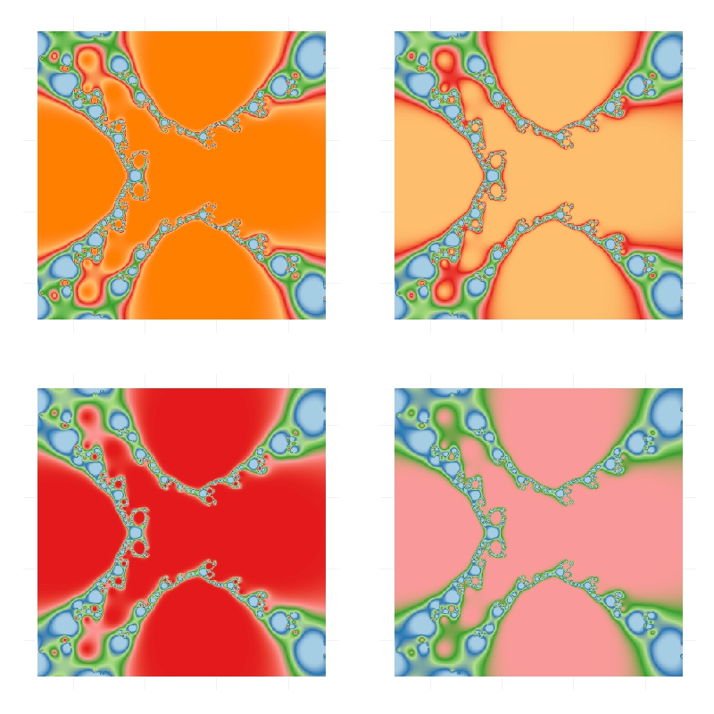
Andy Warhol was mathematician. At least, he knew how clustering algorithms work. I am pretty sure of this after doing this experiment.  First of all, let me introduce you to the breathtaking Grace Kelly:

936full-grace-kelly

In my previous post I worked also with images showing how simple is to operate with them since they are represented by matrices. This is another example of this. Third dimension of an image matrix is an 3D array representing color of pixels in (r, g, b) format. Applying a cluster algorithm over this information generates groups of pixels with similar color. I used cluster package and because of the high size of picture I decided to use clara algorithm which is extremely fast. Apart of its high speed, another advantage of clara is that clusters are represented by real elements of the population, called medoids, instead of being by average individuals as k-means do. It fits very well with my purposes because once clusters are calculated I only have to change each pixel by its medoid and plot it. Setting clara to divide pixels into 2 groups, generates a 2 colored image. Setting it to 3 groups, generates a 3 colored one and so on. Following, you can find results from 2 to 7 groups:

Warholing2 Warholing3 Warholing4
Warholing5 Warholing6 Warholing7

Working with samples can be a handicap, maybe less important than the speed it produces. Sometimes images generated by n groups seems to be worse fitted than the one generated by n-1 groups. You can see it in this video, where results from 1 to 60 groups are presented sequentially. It only takes 42 seconds.

Here you have the code. Feel free to warholing:

library("biOps")
library("abind")
library("reshape")
library("reshape2")
library("cluster")
library("sp")
#######################################################################################################
#Initialization
#######################################################################################################
x     <- readJpeg("936full-grace-kelly.jpg")
plot(x)
#######################################################################################################
#Data
#######################################################################################################
data <- merge(merge(melt(x[,,1]), melt(x[,,2]), by=c("X1", "X2")), melt(x[,,3]), by=c("X1", "X2"))
colnames(data) <- c("X1", "X2", "r", "g", "b")
#######################################################################################################
#Clustering
#######################################################################################################
colors <- 5
clarax <- clara(data[,3:5], colors)
datacl   <- data.frame(data, clarax$cluster)
claradf2 <- as.data.frame(clarax$medoids)
claradf2$id <- as.numeric(rownames(claradf2))
colnames(claradf2) <- c("r", "g", "b", "clarax.cluster")
claradf <- merge(datacl, claradf2, by=c("clarax.cluster"))
colnames(claradf) <-c("clarax.cluster", "X1", "X2", "r.x", "g.x", "b.x", "r.y", "g.y", "b.y")
datac <- claradf[do.call("order", claradf[c("X1", "X2")]), ]
x1<-acast(datac[,c(2,3,7)], X1~X2, value.var="r.y") 
x2<-acast(datac[,c(2,3,8)], X1~X2, value.var="g.y") 
x3<-acast(datac[,c(2,3,9)], X1~X2, value.var="b.y") 
warhol <- do.call(abind, c(list(x1,x2,x3), along = 3))
plot(imagedata(warhol))
writeJpeg(paste("Warholing", as.character(colors), ".jpg", sep=""), imagedata(warhol))