Tag Archives: fractals

The Chaos Game: an experiment about fractals, recursivity and creative coding

Mathematics, rightly viewed, possesses not only truth, but supreme beauty (Bertrand Russell)

You have a pentagon defined by its five vertex. Now, follow these steps:

  • Step 0: take a point inside the pentagon (it can be its center if you want to do it easy). Keep this point in a safe place.
  • Step 1: choose a vertex randomly and take the midpoint between both of them (the vertex and the original point). Keep also this new point. Repeat Step 1 one more time.
  • Step 2: compare the last two vertex that you have chosen. If they are the same, choose another with this condition: if it’s not a neighbor of the last vertex you chose, keep it. If it is a neighbor, choose another vertex randomly until you choose a not-neighbor one. Then, take the midpoint between the last point you obtained and this new vertex. Keep also this new point.
  • Step 3: Repeat Step 2 a number of times and after that, do a plot with the set of points that you obtained.

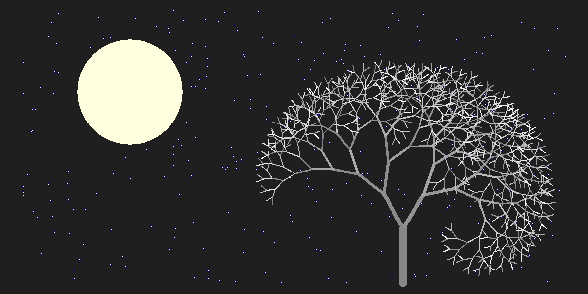
If you repeat these steps 10 milion times, you will obtain this stunning image:

I love the incredible ability of maths to create beauty. More concretely, I love the fact of how repeating extremely simple operations can bring you to unexpected places. Would you expect that the image created with the initial naive algorithm would be that? I wouldn’t. Even knowing the result I cannot imagine how those simple steps can produce it.

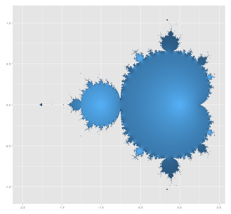
The image generated by all the points repeat itself at different scales. This characteristic, called self-similarity, is property of fractals and make them extremely attractive. Step 2 is the key one to define the shape of the image. Apart of comparing two previous vertex as it’s defined in the algorithm above, I implemented two other versions:

  • one version where the currently chosen vertex cannot be the same as the previously chosen vertex.
  • another one where the currently chosen vertex cannot neighbor the previously chosen vertex if the three previously chosen vertices are the same (note that this implementation is the same as the original but comparing with three previous vertex instead two).

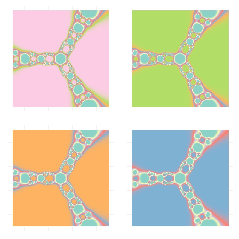
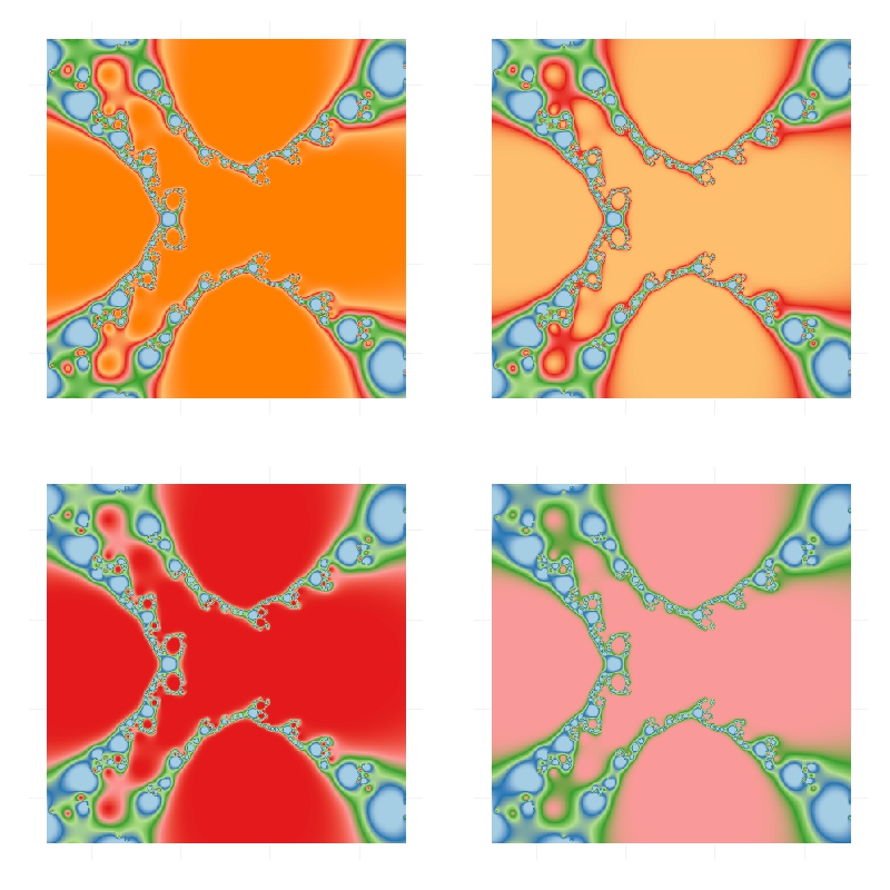
These images are the result of applying the three versions of the algorithm to a square, a pentagon, a hexagon and a heptagon (a row for each polygon and a column for each algorithm):

From a technical point of view I used Rcppto generate the set of points. Since each iteration depends on the previous one, the loop cannot easily vectorised and C++ is a perfect option to avoid the bottleneck if you use another technique to iterate. In this case, instead of writing the C++ directly inside the R file with cppFunction(), I used a stand-alone C++ file called chaos_funcs.cpp to write the C++ code that I load into R using sourceCpp().

Some days ago, I gave a tutorial at the coding club of the University Carlos III in Madrid where we worked with the integration of C++ and R to create beautiful images of strange attractors. The tutorial and the code we developed is here. You can also find the code of this experiment here. Enjoy!

Plants

Blue dragonflies dart to and fro
I tie my life to your balloon and let it go
(Warm Foothills, Alt-J)

In my last post I did some drawings based on L-Systems. These drawings are done sequentially. At any step, the state of the drawing can be described by the position (coordinates) and the orientation of the pencil. In that case I only used two kind of operators: drawing a straight line and turning a constant angle. Today I used two more symbols to do stack operations:

  • “[“ Push the current state (position and orientation) of the pencil onto a pushdown
    operations stack
  • “]” Pop a state from the stack and make it the current state of the pencil (no line is drawn)

These operators allow to return to a previous state to continue drawing from there. Using them you can draw plants like these:

Each image corresponds to a different axiom, rules, angle and depth. I described these terms in my previous post. If you want to reproduce them you can find the code below (each image corresponds to a different set of axiom, rules, angle and depth parameters). Change colors, add noise to angles, try your own plants … I am sure you will find nice images:


library(gsubfn)
library(stringr)
library(dplyr)
library(ggplot2)

#Plant 1
axiom="F"
rules=list("F"="FF-[-F+F+F]+[+F-F-F]")
angle=22.5
depth=4

#Plant 2
axiom="X"
rules=list("X"="F[+X][-X]FX", "F"="FF")
angle=25.7
depth=7

#Plant 3
axiom="X"
rules=list("X"="F[+X]F[-X]+X", "F"="FF")
angle=20
depth=7

#Plant 4
axiom="X"
rules=list("X"="F-[[X]+X]+F[+FX]-X", "F"="FF")
angle=22.5
depth=5

#Plant 5
axiom="F"
rules=list("F"="F[+F]F[-F]F")
angle=25.7
depth=5

#Plant 6
axiom="F"
rules=list("F"="F[+F]F[-F][F]")
angle=20
depth=5


for (i in 1:depth) axiom=gsubfn(".", rules, axiom)

actions=str_extract_all(axiom, "\\d*\\+|\\d*\\-|F|L|R|\\[|\\]|\\|") %>% unlist

status=data.frame(x=numeric(0), y=numeric(0), alfa=numeric(0))
points=data.frame(x1 = 0, y1 = 0, x2 = NA, y2 = NA, alfa=90, depth=1)


for (action in actions) 
{
  if (action=="F")
  {
    x=points[1, "x1"]+cos(points[1, "alfa"]*(pi/180))
    y=points[1, "y1"]+sin(points[1, "alfa"]*(pi/180))
    points[1,"x2"]=x
    points[1,"y2"]=y
    data.frame(x1 = x, y1 = y, x2 = NA, y2 = NA, 
               alfa=points[1, "alfa"],
               depth=points[1,"depth"]) %>% rbind(points)->points
  }
  if (action %in% c("+", "-")){
    alfa=points[1, "alfa"]
    points[1, "alfa"]=eval(parse(text=paste0("alfa",action, angle)))
  }
  if(action=="["){ 
    data.frame(x=points[1, "x1"], y=points[1, "y1"], alfa=points[1, "alfa"]) %>% 
      rbind(status) -> status
    points[1, "depth"]=points[1, "depth"]+1
  }
  
  if(action=="]"){ 
    depth=points[1, "depth"]
    points[-1,]->points
    data.frame(x1=status[1, "x"], y1=status[1, "y"], x2=NA, y2=NA, 
               alfa=status[1, "alfa"],
               depth=depth-1) %>% 
      rbind(points) -> points
    status[-1,]->status
  }
}

ggplot() + 
  geom_segment(aes(x = x1, y = y1, xend = x2, yend = y2), 
               lineend = "round", 
               colour="white",
               data=na.omit(points)) + 
  coord_fixed(ratio = 1) +
  theme(legend.position="none",
        panel.background = element_rect(fill="black"),
        panel.grid=element_blank(),
        axis.ticks=element_blank(),
        axis.title=element_blank(),
        axis.text=element_blank())

The Pythagorean Tree Is In Bloom

There is geometry in the humming of the strings, there is music in the spacing of the spheres (Pythagoras)

Spring is here and I will be on holiday next week. I cannot be more happy! It is time to celebrate so I have drawn another fractal. It is called the Pythagorean Tree:

PythagoreanTree

Here you have the code. See you soon:

library("grid")
l=0.15 #Length of the square
grid.newpage()
gr <- rectGrob(width=l, height=l, name="gr") #Basic Square
pts <- data.frame(level=1, x=0.5, y=0.1, alfa=0) #Centers of the squares
for (i in 2:10) #10=Deep of the fractal. Feel free to change it
{
  df<-pts[pts$level==i-1,]
  for (j in 1:nrow(df))
  {
    pts <- rbind(pts, 
                 c(i, 
                   df[j,]$x-2*l*((1/sqrt(2))^(i-1))*sin(df[j,]$alfa+pi/4)-0.5*l*((1/sqrt(2))^(i-2))*sin(df[j,]$alfa+pi/4-3*pi/4), 
                   df[j,]$y+2*l*((1/sqrt(2))^(i-1))*cos(df[j,]$alfa+pi/4)+0.5*l*((1/sqrt(2))^(i-2))*cos(df[j,]$alfa+pi/4-3*pi/4),                  
                   df[j,]$alfa+pi/4))
    pts <- rbind(pts, 
                 c(i, 
                   df[j,]$x-2*l*((1/sqrt(2))^(i-1))*sin(df[j,]$alfa-pi/4)-0.5*l*((1/sqrt(2))^(i-2))*sin(df[j,]$alfa-pi/4+3*pi/4), 
                   df[j,]$y+2*l*((1/sqrt(2))^(i-1))*cos(df[j,]$alfa-pi/4)+0.5*l*((1/sqrt(2))^(i-2))*cos(df[j,]$alfa-pi/4+3*pi/4),                  
                   df[j,]$alfa-pi/4))
  }
}
for (i in 1:nrow(pts))
{
  grid.draw(editGrob(gr, vp=viewport(x=pts[i,]$x, y=pts[i,]$y, w=((1/sqrt(2))^(pts[i,]$level-1)), h=((1/sqrt(2))^(pts[i,]$level-1)), angle=pts[i,]$alfa*180/pi), 
            gp=gpar(col=0, lty="solid", fill=rgb(139*(nrow(pts)-i)/(nrow(pts)-1), 
                                                 (186*i+69*nrow(pts)-255)/(nrow(pts)-1), 
                                                  19*(nrow(pts)-i)/(nrow(pts)-1), 
                                                  alpha= (-110*i+200*nrow(pts)-90)/(nrow(pts)-1), max=255))))
}

Blurry Fractals

Beauty is the first test; there is no permanent place in the world for ugly mathematics (G. H. Hardy)

Newton basin fractals are the result of iterating Newton’s method to find roots of a polynomial over the complex plane. It maybe sound a bit complicated but is actually quite simple to understand. Those who would like to read some more about Newton basin fractals can visit this page.

This fractals are very easy to generate in R and produce very nice images. Making a small number of iterations, resulting images seems to be blurred when are represented with tile geometry in ggplot. Combined with palettes provided by RColorBrewer give rise to very interesting images. Here you have some examples:

Result for f(z)=z3-1 and palette equal to Set3:Blurry1-Set3Result for f(z)=z4+z-1 and palette equal to Paired:Blurry2-PairedResult for f(z)=z5+z3+z-1 and palette equal to Dark2:Blurry3-Dark2Here you have the code. If you generate nice pictures I will be very grateful if you send them to me:

library(ggplot2)
library(numDeriv)
library(RColorBrewer)
library(gridExtra)
## Polynom: choose only one or try yourself
f  <- function (z) {z^3-1}        #Blurry 1
#f  <- function (z) {z^4+z-1}     #Blurry 2
#f  <- function (z) {z^5+z^3+z-1} #Blurry 3
z <- outer(seq(-2, 2, by = 0.01),1i*seq(-2, 2, by = 0.01),'+')
for (k in 1:5) z <- z-f(z)/matrix(grad(f, z), nrow=nrow(z))
## Supressing texts, titles, ticks, background and legend.
opt <- theme(legend.position="none",
             panel.background = element_blank(),
             axis.ticks=element_blank(), 
             axis.title=element_blank(), 
             axis.text =element_blank())
z <- data.frame(expand.grid(x=seq(ncol(z)), y=seq(nrow(z))), z=as.vector(exp(-Mod(f(z)))))
# Create plots. Choose a palette with display.brewer.all()
p1 <- ggplot(z, aes(x=x, y=y, color=z)) + geom_tile() + scale_colour_gradientn(colours=brewer.pal(8, "Paired")) + opt
p2 <- ggplot(z, aes(x=x, y=y, color=z)) + geom_tile() + scale_colour_gradientn(colours=brewer.pal(7, "Paired")) + opt
p3 <- ggplot(z, aes(x=x, y=y, color=z)) + geom_tile() + scale_colour_gradientn(colours=brewer.pal(6, "Paired")) + opt
p4 <- ggplot(z, aes(x=x, y=y, color=z)) + geom_tile() + scale_colour_gradientn(colours=brewer.pal(5, "Paired")) + opt
# Arrange four plots in a 2x2 grid
grid.arrange(p1, p2, p3, p4, ncol=2)

The Lonely Acacia Is Rocked By The Wind Of The African Night

If you can walk you can dance. If you can talk you can sing (Zimbabwe Proverb)

There are two things in this picture I would like to emphasise. First one is that everything is made using points and lines. The moon is an enormous point, stars are three small nested points and the tree is a set of straight lines. Points and lines over a simple cartesian graph, no more. Second one is that the tree is a jittered fractal. In particular, is a jittered L-system fractal, a formalism invented in 1968 by a biologist (Aristid Lindemayer) that yields a mathematical description of plan growth. Why jittered? Because I add some positive noise to the angle in which branches are divided by two iteratively. It gives to the tree the sense to be rocked by the wind. This is the picture:

image1

I generated 120 images and gathered in this video to make the wind happen. The stunning song is called Kothbiro performed by Ayub Ogada.

Here you have the code:

depth <- 9
angle<-30 #Between branches division
L <- 0.90 #Decreasing rate of branches by depth
nstars <- 300 #Number of stars to draw
mstars <- matrix(runif(2*nstars), ncol=2)
branches <- rbind(c(1,0,0,abs(jitter(0)),1,jitter(5, amount = 5)), data.frame())
colnames(branches) <- c("depth", "x1", "y1", "x2", "y2", "inertia")
for(i in 1:depth)
{
  df <- branches[branches$depth==i,]
  for(j in 1:nrow(df))
  {
    branches <- rbind(branches, c(df[j,1]+1, df[j,4], df[j,5], df[j,4]+L^(2*i+1)*sin(pi*(df[j,6]+angle)/180), df[j,5]+L^(2*i+1)*cos(pi*(df[j,6]+angle)/180), df[j,6]+angle+jitter(10, amount = 8)))
    branches <- rbind(branches, c(df[j,1]+1, df[j,4], df[j,5], df[j,4]+L^(2*i+1)*sin(pi*(df[j,6]-angle)/180), df[j,5]+L^(2*i+1)*cos(pi*(df[j,6]-angle)/180), df[j,6]-angle+jitter(10, amount = 8)))
  }
}
nodes <- rbind(as.matrix(branches[,2:3]), as.matrix(branches[,4:5]))
png("image.png", width = 1200, height = 600)
plot.new()
par(mai = rep(0, 4), bg = "gray12")
plot(nodes, type="n", xlim=c(-7, 3), ylim=c(0, 5))
for (i in 1:nrow(mstars)) 
{
  points(x=10*mstars[i,1]-7, y=5*mstars[i,2], col = "blue4", cex=.7, pch=16)
  points(x=10*mstars[i,1]-7, y=5*mstars[i,2], col = "blue",  cex=.3, pch=16)
  points(x=10*mstars[i,1]-7, y=5*mstars[i,2], col = "white", cex=.1, pch=16)
}
# The moon
points(x=-5, y=3.5, cex=40, pch=16, col="lightyellow")
# The tree
for (i in 1:nrow(branches)) {lines(x=branches[i,c(2,4)], y=branches[i,c(3,5)], col = paste("gray", as.character(sample(seq(from=50, to=round(50+5*branches[i,1]), by=1), 1)), sep = ""), lwd=(65/(1+3*branches[i,1])))}
rm(branches)
dev.off()

I Need A New Computer To Draw Fractals!

Computer Science is no more about computers than astronomy is about telescopes (E. W. Dijkstra)

Some days ago I published a post about how to build fractals with R using Multiple Reduction Copt Machine (MRCM) algorithm. Is that case I used a feature of the grid package that allows you to locate objects easily into the viewPort avoiding to work with coordinates. It does not work well if you want to divide your seed image into five subimages located in the vertex of a regular pentagon. No problem: after refreshing some trigonometric formulas and after understanding how to work with coordinates I felt strong enough to program the Final-MRCM-Fractal-Builder. But here comes the harsh reality. My computer crashes when I try to go beyond five degrees of depth. Imposible. In the example of Sierpinski’s triangle, where every square in divided into three small ones, I reached seven degrees of depth. I am deeply frustrated. These are drawings for 1, 2, 3 and 5 degrees of depth.

Rplot01c Rplot02c Rplot03cRplot05c

Please, if someone modifies code to make it more efficient, let me know. I used circles in this case instead squares. Here you have it:

library(grid)
grid.newpage()
rm(list = ls())
ratio <- 0.4
pmax <- 5 # Depth
vp1 <- viewport(w=1, h=1)
vp2 <- viewport(w=ratio, h=ratio, just=c(0.75*sin(2*pi*1/5)+0.5, 0.75*cos(2*pi*1/5)+0.75*pi*1/5))
vp3 <- viewport(w=ratio, h=ratio, just=c(0.75*sin(2*pi*0/5)+0.5, 0.75*cos(2*pi*0/5)+0.75*pi*1/5))
vp4 <- viewport(w=ratio, h=ratio, just=c(0.75*sin(2*pi*2/5)+0.5, 0.75*cos(2*pi*2/5)+0.75*pi*1/5))
vp5 <- viewport(w=ratio, h=ratio, just=c(0.75*sin(2*pi*3/5)+0.5, 0.75*cos(2*pi*3/5)+0.75*pi*1/5))
vp6 <- viewport(w=ratio, h=ratio, just=c(0.75*sin(2*pi*4/5)+0.5, 0.75*cos(2*pi*4/5)+0.75*pi*1/5))
pushViewport(vp1)
grid.rect(gp=gpar(fill="white", col=NA))
m <- as.matrix(expand.grid(rep(list(2:6), pmax)))
for (j in 1:nrow(m))
{
for(k in 1:ncol(m)) {pushViewport(get(paste("vp",m[j,k],sep="")))}
grid.circle(gp=gpar(col="dark grey", lty="solid", fill=rgb(sample(0:255, 1),sample(0:255, 1),sample(0:255, 1), alpha= 95, max=255)))
upViewport(pmax)
}

What The Hell Is Pi Doing Here?

Nothing in Nature is random … A thing appears random only through the incompleteness of our knowledge (Benedict Spinoza)

This is one of my favorite mathematical mysteries. In 1991 David Boll was trying to confirm that the neck of the Mandelbrot Set is 0 in thickness. Neck is located at -0.75+0i (where two biggest circles meet each other). Mandelbrot50He tried with complex numbers like -0.75+εi for small values of ε demonstrating the divergence of all these numbers. And here comes the mystery: multiplying ε and the corresponding number of iterations it took for the iterate to diverge, gives an approximation of π that is within ±ε. Is not fascinating? I replicated David Boll’s experiment for positive and negative values of ε. I draw results as follows:

mandelbrot

Before doing it, I thought I was going to find some pattern in the graphic. Apart from the mirror effect produced by the sign of ε, there is nothing recognizable. Convergence is chaotic. Here you have the code. This example is also nice to practice with ggplot2 package, one of the totems of R:

i<-0    # Counter of iterations
x  <- 0 # Initialization
while (Mod(x) <= 2)
{
x <- x^2+(c+complex(real = 0, imaginary = e))
i <- i+1
}
i
}
results <- as.data.frame(c(NULL,NULL))
for (j in 1:length(epsilons))
{results <- rbind(results, c(epsilons[j], testMSConvergence(epsilons[j])))}
colnames(results) <- c('epsilon', 'iterations')
dev.off()
p <- ggplot(results, aes(epsilon,abs(epsilon)*iterations))+
xlab("epsilon")+
ylab("abs(epsilon)*iterations")+
opts(axis.title.x=theme_text(size=16)) +
opts(axis.title.y=theme_text(size=16)) +
ggtitle("How to Estimate Pi Using Mandelbrot Set's Neck")+
theme(plot.title = element_text(size=20, face="bold"))
p <- p + geom_ribbon(data=results,aes(ymin=abs(epsilon)*iterations-abs(epsilon),ymax=abs(epsilon)*iterations+abs(epsilon)), alpha=0.3)
p <- p + geom_abline(intercept = pi, , slope = 0, size = 0.4, linetype=2, colour = "black", alpha=0.8)
p <- p + geom_line(colour = "dark blue", size = 1, linetype = 1)
p <- p + geom_text(x = 0, y = pi, label="pi", vjust=2, colour="dark blue")
p <- p + geom_point(x = 0, y = pi, size = 6, colour="dark blue")
p + geom_point(x = 0, y = pi, size = 4, colour="white")

Building Affine Transformation Fractals With R

Clouds are not spheres, mountains are not cones, coastlines are not circles and bark is not smooth, nor does lightning travel in a straight line (Benoit Maldelbrot)

Fractals are beautiful, hypnotics, mysterious. Cantor set has as many points as the real number line but has zero measure. After 100 steps, the Koch curve created from a 1 inch segment is long enough  to wrap around the Earth at the equator nearly four thousand times. The Peano Curve is a line that has the same dimension as a plane. Fractals are weird mathematical objects. Fractals are very cool.

One way to build fractals is using the Multiple Reduction Copy Machine (MRCM) algorithm which uses affine linear transformations over a seed image to build fractals. MRCM are iterative algorithms that perform some sort of copy+paste task. The idea is quite simple: take a seed image, transform it (clonation, scalation, rotation), obtain the new image and iterate.

To create the Sierpinsky Gasket Fractal you part from a square. Then you divide it into three smaller squares, locate them as a pyramid and iterate doing the same with avery new square created. Making these things is very easy with grid package. Defining the division (i.e. the affine transformation) properly using viewPort function and navigating between them is all you need. Here you have the Sierpinsky Gasket Fractal with 1, 3, 5 and 7 levels of depth. I filled in squares with random colours (I like giving some touch of randomness to pictures). Here you have pictures:

Rplot01 Rplot03

Rplot05 Rplot07

And here you have the code. Feel free to build your own fractals.

library(grid)
rm(list = ls())
grid.newpage()
pmax <- 5 # Depth of the fractal
vp1=viewport(x=0.5,y=0.5,w=1, h=1)
vp2=viewport(w=0.5, h=0.5, just=c("centre", "bottom"))
vp3=viewport(w=0.5, h=0.5, just=c("left", "top"))
vp4=viewport(w=0.5, h=0.5, just=c("right", "top"))
pushViewport(vp1)
m <- as.matrix(expand.grid(rep(list(2:4), pmax)))
for (j in 1:nrow(m))
{
for(k in 1:ncol(m)) {pushViewport(get(paste("vp",m[j,k],sep="")))}
grid.rect(gp=gpar(col="dark grey", lty="solid",
fill=rgb(sample(0:255, 1),sample(0:255, 1),sample(0:255, 1), alpha= 95, max=255)))
upViewport(pmax)
}