Tag Archives: imager

Clustering Frankenstein

Necesito para estar sentado, un arbolito en este descampado (Desarraigo, Extremoduro)

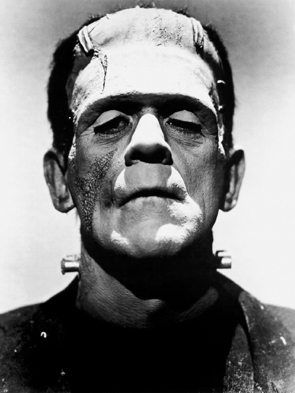
From time to time I come back to experiment with this stunning photograph of Boris Karloff as Frankenstein’s monster. I have done several of them previously: from decomposing it into Voronoi regions, to draw it as a single line portrait using an algorithm to solve the travelling salesman problem. I also used this last technique to do a pencil portrait of the image. Today I will use a machine learning algorithm to reinterpret the monster once again. Concretely, I will use hierarchical clustering to do drawings like this one:

The idea is simple: once loaded the photograph, the first step is to binarize it into a black and white image using thresold function of imager package. After that, a random sample of black points is taken. Here comes the clustering algorithm, which starts measuring the euclidean distance between each pair of points. Then, a hierarchical clustering is done so I can reproduce how points are gathered walking through the resulting dendrogram of the previous clustering, starting from the maximum number of clusters (each cluster is an individual point) and ending with the minimum one (just one cluster with the whole sample). The next image shows and example of this process for a sample of 25 points. The left plot shows the population of points and the right one the way that points are connected once the dendrogram is analyzed following the steps described before:

Applying this technique to a big amount of points (between 2.000 and 5.000) result in very interesting drawings. To make process faster, I used map function from purrr package. To render the graph I use ggplot function with geom_curve. This geometry draws a curve between two points, named (x, y) and (xend, yend) respectively. Among others, there are two important parameters to control its shape: curvature (negative values produce left-hand curves, positive values produce right-hand curves, and zero produces a straight line) and angle (values less than 90 skew the curve towards the start point and values greater than 90 skew the curve towards the end point). Playing with this paramaters, as well as with the sample size, you can generate a wide variety of drawings (note that here only appear the segments, since now I removed the points of their extremes):

You can find the code of this experiment here. If you do something interesting with it, please let me know. Thanks a lot for reading my post.

Pencil Scribbles

Con las bombas que tiran los fanfarrones, se hacen las gaditanas tirabuzones (Palma y corona, Carmen Linares)

This time I draw Franky again using an algorithm to solve the Travelling Salesman Problem as I did in my last post. On this occasion, instead of doing just one single line drawing, I overlap many of them (250 concretely), each of them sampling 400 points on the original image (in my previous post I sampled 8.000 points). Last difference is that I don’t convert the image to pure black and white with threshold function: now I use the gray scale number of each pixel to weight the sample.

Once again, I use ggplot2 package, and its magical geom_path, to generate the image. The pencil effect is obtained giving a very high transparency to the lines. This is the result:

I love when someone else experiment with my experiments as Mara Averick did:

Or Erik-Jan van Kesteren:

You can do it as well with this one, since you will find the code here. Please, let me know your own creations if you do. You can find me on twitter or by email.

P.S.: Although it may seems otherwise, I’m not obsessed with Frankenstein 🙂

The Travelling Salesman Portrait

I have noticed even people who claim everything is predestined, and that we can do nothing to change it, look before they cross the road (Stephen Hawking)

Imagine a salesman and a set of cities. The salesman has to visit each one of the cities starting from a certain one and returning to the same city. The challenge is finding the route which minimizes the total length of the trip. This is the Travelling Salesman Problem (TSP): one of the most profoundly studied questions in computational mathematics. Since you can find a huge amount of articles about the TSP in the Internet, I will not give more details about it here.

In this experiment I apply an heuristic algorithm to solve the TSP to draw a portrait. The idea is pretty simple:

  • Load a photo
  • Convert it to black and white
  • Choose a sample of black points
  • Solve the TSP to calculate a route among the points
  • Plot the route

The result is a single line drawing of the image that you loaded. To solve the TSP I used the arbitrary insertion heuristic algorithm (Rosenkrantz et al. 1977), which is quite efficient.

To illustrate the idea, I have used again this image of Frankenstein (I used it before in this other experiment). This is the result:

You can find the code here.

Frankenstein

Remember me, remember me, but ah! forget my fate (Dido’s Lament, Henry Purcell)

A Voronoi diagram divides a plane based on a set of original points. Each polygon, or Voronoi cell, contains an original point and all that are closer to that point than any other.

This is a nice example of a Voronoi tesselation. You can find good explanations of Voronoi diagrams and Delaunay triangulations here (in English) or here (in Spanish).

A grayscale image is simply a matrix where darkness of pixel located in coordinates (i, j) is represented by the value of its corresponding element of the matrix: a grayscale image is a dataset. This is a Voronoi diagraman of Frankenstein:

To do it I followed the next steps:

  1. Read this image
  2. Convert it to gray scale
  3. Turn it into a pure black and white image
  4. Obtain a random sample of black pixels (previous image corresponds to a sample of 6.000 points)
  5. Computes the Voronoi tesselation

Steps 1 to 3 were done with imager, a very appealing package to proccess and analice images. Step 5 was done with deldir, also a convenient package which computes Delaunay triangulation and the Dirichlet or Voronoi tessellations.

The next grid shows tesselations for sample size from 500 to 12.000 points and step equal to 500:

I gathered all previous images in this gif created with magick, another amazing package of R I discovered recently:

This is the code:

library(imager)
library(dplyr)
library(deldir)
library(ggplot2)
library(scales)

# Download the image
file="http://ereaderbackgrounds.com/movies/bw/Frankenstein.jpg"
download.file(file, destfile = "frankenstein.jpg", mode = 'wb')

# Read and convert to grayscale
load.image("frankenstein.jpg") %>% grayscale() -> x

# This is just to define frame limits
x %>% 
  as.data.frame() %>% 
  group_by() %>% 
  summarize(xmin=min(x), xmax=max(x), ymin=min(y), ymax=max(y)) %>% 
  as.vector()->rw

# Filter image to convert it to bw
x %>%
  threshold("45%") %>% 
  as.cimg() %>% 
  as.data.frame() -> df

# Function to compute and plot Voronoi tesselation depending on sample size
doPlot = function(n)
{
  #Voronoi tesselation
  df %>% 
  sample_n(n, weight=(1-value)) %>% 
  select(x,y) %>% 
  deldir(rw=rw, sort=TRUE) %>% 
  .$dirsgs -> data

  # This is just to add some alpha to lines depending on its longitude
  data %>% 
    mutate(long=sqrt((x1-x2)^2+(y1-y2)^2),
         alpha=findInterval(long, quantile(long, probs = seq(0, 1, length.out = 20)))/21)-> data

  # A little bit of ggplot to plot results
  data %>% 
    ggplot(aes(alpha=(1-alpha))) +
    geom_segment(aes(x = x1, y = y1, xend = x2, yend = y2), color="black", lwd=1) +
    scale_x_continuous(expand=c(0,0))+
    scale_y_continuous(expand=c(0,0), trans=reverse_trans())+
    theme(legend.position  = "none",
            panel.background = element_rect(fill="white"),
            axis.ticks       = element_blank(),
            panel.grid       = element_blank(),
            axis.title       = element_blank(),
            axis.text        = element_blank())->plot

return(plot)
}

# I call the previous function and store resulting plot in jpeg format
i=5000
name=paste0("frankie",i,".jpeg")
jpeg(name, width = 600, height = 800, units = "px", quality = 100)
doPlot(i)
dev.off()

# Once all images are stored I can create gif
library(magick)
frames=c()
images=list.files(pattern="jpeg")

for (i in length(images):1)
{
  x=image_read(images[i])
  x=image_scale(x, "300")
  c(x, frames) -> frames
}
animation=image_animate(frames, fps = 2)
image_write(animation, "Frankenstein.gif")