Tag Archives: biOps

Warholing Grace With Clara

Do not believe anything: what artists really do is to hang around all day (Paco de Lucia)

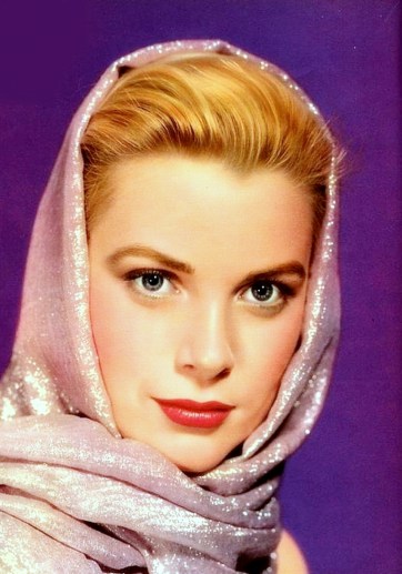
Andy Warhol was mathematician. At least, he knew how clustering algorithms work. I am pretty sure of this after doing this experiment.  First of all, let me introduce you to the breathtaking Grace Kelly:

936full-grace-kelly

In my previous post I worked also with images showing how simple is to operate with them since they are represented by matrices. This is another example of this. Third dimension of an image matrix is an 3D array representing color of pixels in (r, g, b) format. Applying a cluster algorithm over this information generates groups of pixels with similar color. I used cluster package and because of the high size of picture I decided to use clara algorithm which is extremely fast. Apart of its high speed, another advantage of clara is that clusters are represented by real elements of the population, called medoids, instead of being by average individuals as k-means do. It fits very well with my purposes because once clusters are calculated I only have to change each pixel by its medoid and plot it. Setting clara to divide pixels into 2 groups, generates a 2 colored image. Setting it to 3 groups, generates a 3 colored one and so on. Following, you can find results from 2 to 7 groups:

Warholing2 Warholing3 Warholing4
Warholing5 Warholing6 Warholing7

Working with samples can be a handicap, maybe less important than the speed it produces. Sometimes images generated by n groups seems to be worse fitted than the one generated by n-1 groups. You can see it in this video, where results from 1 to 60 groups are presented sequentially. It only takes 42 seconds.

Here you have the code. Feel free to warholing:

library("biOps")
library("abind")
library("reshape")
library("reshape2")
library("cluster")
library("sp")
#######################################################################################################
#Initialization
#######################################################################################################
x     <- readJpeg("936full-grace-kelly.jpg")
plot(x)
#######################################################################################################
#Data
#######################################################################################################
data <- merge(merge(melt(x[,,1]), melt(x[,,2]), by=c("X1", "X2")), melt(x[,,3]), by=c("X1", "X2"))
colnames(data) <- c("X1", "X2", "r", "g", "b")
#######################################################################################################
#Clustering
#######################################################################################################
colors <- 5
clarax <- clara(data[,3:5], colors)
datacl   <- data.frame(data, clarax$cluster)
claradf2 <- as.data.frame(clarax$medoids)
claradf2$id <- as.numeric(rownames(claradf2))
colnames(claradf2) <- c("r", "g", "b", "clarax.cluster")
claradf <- merge(datacl, claradf2, by=c("clarax.cluster"))
colnames(claradf) <-c("clarax.cluster", "X1", "X2", "r.x", "g.x", "b.x", "r.y", "g.y", "b.y")
datac <- claradf[do.call("order", claradf[c("X1", "X2")]), ]
x1<-acast(datac[,c(2,3,7)], X1~X2, value.var="r.y") 
x2<-acast(datac[,c(2,3,8)], X1~X2, value.var="g.y") 
x3<-acast(datac[,c(2,3,9)], X1~X2, value.var="b.y") 
warhol <- do.call(abind, c(list(x1,x2,x3), along = 3))
plot(imagedata(warhol))
writeJpeg(paste("Warholing", as.character(colors), ".jpg", sep=""), imagedata(warhol))
Face To Face With Marilyn Monroe

Symmetry is what we see at a glance (Blaise Pascal)

Ladies and gentlement, the beautiful Marilyn Monroe:

marilyn-monroe3

There are several image processing packages in R. In this experiment I used biOps, which turns images into 3D matrices. The third dimension is a 3-array corresponding to (r, g, b) color of pixel defined by two other dimensions. Since images are defined by matrices, you can do simple operations to produce interesting images from the original one. For example, this is what happens swaping last half of columns by first one and preserving its order:

IMG01-Interchange

It is also very simple to generate two artificial symmetrical faces matching each half with itself as a mirror. By the way, I prefer the first one: maybe two sexy moles are better than just one.

IMG03-Symmetric2 IMG02-Symmetric1

Let’s introduce a bit of randomness. This is what happens when you take an uniform sample of rows and columns (first image) or an uniform sample of pixels of the image (second one):

IMG04-Uniform1 IMG05-Uniform2

And this is what happens when you divide image into blocks and mix them randomly:

IMG07-Mosaic

There is a funny and useful function called jitter which adds a small amount of noise to a numeric vector. What happens when you jitter every pixel of the image? As you can see, It becomes very vintage:

IMG06-Jitter

What if you transpose matrix? What if you change every color by another one? What if you change only a small range of them? What if you sum two images? What if you translate rgb colors into a grey scale? What if …? I answered some of these questions already and results are nice as well. After all, Marilyn can be represented as a simple matrix. Or maybe not.

Make your own experiments:

library("biOps")
library("abind")
#############################################################
#Read Original Image
#############################################################
x     <- readJpeg("marilyn-monroe3.jpg")
plot(x)
#############################################################
#1. Swap
#############################################################
plot(imagedata(abind(x[,(ncol(x)/2):ncol(x),], x[,1:(ncol(x)/2),] , along=2)))
dev.copy(jpeg,filename="IMG01-Swap.jpg");
dev.off ();
#############################################################
#2. Artificial Symmetrical faces
#############################################################
plot(imagedata(abind(x[,1:(ncol(x)/2),], x[,(ncol(x)/2):1,] , along=2)))
dev.copy(jpeg,filename="IMG02-Symmetric1.jpg");
dev.off ();
plot(imagedata(abind(x[,ncol(x):(ncol(x)/2),], x[,(ncol(x)/2):ncol(x),] , along=2)))
dev.copy(jpeg,filename="IMG03-Symmetric2.jpg");
dev.off ();
#############################################################
#3. Uniform sampling over axis points
#############################################################
x2   <- aperm(array(255, dim = c(3, ncol(x), nrow(x))))
rows <- sample(1:nrow(x), round(nrow(x)*0.80), replace = FALSE)
cols <- sample(1:ncol(x), round(ncol(x)*0.80), replace = FALSE)
for (i in 1:length(rows)) 
{
  for (j in 1: length(cols)) 
    {
    x2[rows[i], cols[j],1]<-x[rows[i], cols[j],1] 
    x2[rows[i], cols[j],2]<-x[rows[i], cols[j],2] 
    x2[rows[i], cols[j],3]<-x[rows[i], cols[j],3] 
  }
}
plot(imagedata(x2))
dev.copy(jpeg,filename="IMG04-Uniform1.jpg");
dev.off ();
#############################################################
#4. Uniform sampling over pixels
#############################################################
m2 <- matrix(rbinom(nrow(x)*ncol(x),1,0.5),nrow(x),ncol(x))
x4<- do.call(abind, c(list(x[,,1]*m2+(m2==0)*255,x[,,2]*m2+(m2==0)*255,x[,,3]*m2+(m2==0)*255), along = 3))
plot(imagedata(x4))
dev.copy(jpeg,filename="IMG05-Uniform2.jpg");
dev.off ();
#############################################################
#6. Jittering
#############################################################
x1<-mapply(as.matrix(x[,,1]), FUN=function(x) 
  {z<-round(x+jitter(0, amount=50)) 
  if(z<0|z>255) x else z})
x1 <- matrix(x1, nrow = nrow(x),ncol = ncol(x))
x2<-mapply(as.matrix(x[,,2]), FUN=function(x) 
{z<-round(x+jitter(0, amount=50)) 
 if(z<0|z>255) x else z})
x2 <- matrix(x2, nrow = nrow(x),ncol = ncol(x))
x3<-mapply(as.matrix(x[,,3]), FUN=function(x) 
{z<-round(x+jitter(0, amount=50)) 
 if(z<0|z>255) x else z})
x3 <- matrix(x3, nrow = nrow(x),ncol = ncol(x))
x4<- do.call(abind, c(list(x1,x2,x3), along = 3))
plot(imagedata(x4))
dev.copy(jpeg,filename="IMG06-Jitter.jpg");
dev.off ();
#############################################################
#7. Mosaic
#############################################################
sptr <- 6 #Row splits
rnkr <- sample(1:sptr, size = sptr, replace = FALSE)
wthr <- floor(nrow(x)/sptr) #Splits width (row)
rnkr <- as.vector(sapply(rnkr, function (x) rep(x,wthr)))
rnkr <- rnkr*10E6+seq(1, length(rnkr), by=1)
rnkr <- rank(rnkr)
sptc <- round(ncol(x)/wthr)
rnkc <- sample(1:sptc, size = sptc, replace = FALSE)
wthc <- floor(ncol(x)/sptc) #Splits width (row)
rnkc <- as.vector(sapply(rnkc, function (x) rep(x,wthc)))
rnkc <- rnkc*10E6+seq(1, length(rnkc), by=1)
rnkc <- rank(rnkc)
x2<-x[1:length(rnkr),1:length(rnkc),]
x2<-x[rank(rnkr),rank(rnkc),]
plot(imagedata(x2))
dev.copy(jpeg,filename="IMG07-Mosaic.jpg");
dev.off ();