Tag Archives: frakenstein

Colonizing Franky

Y otra vez me arranco despacito, al sentir que nada necesito (Locura transitoria, Extremoduro)

One of my favorite sites in the Internet is algorithmic botany . It’s always a source of inspiration for me. I recently discovered there the space colonization algorithm, concretely in this paper. Originally, the algorithm was developed to simulate leaf venation patterns as well as the branching structure of trees and it works by simulating the competition for space between growing veins (or branches). Given a initial set of attractor points (3.000 points in my case), and a initial node (also a point located randomly inside the picture) the algorithm performs the next steps iteratively:

  • measure distances between attractors and nodes
  • assign the closest node to each attractor
  • keep just those pairs (node, attractor) which distance is between a minimum and maximum
  • normalize and obtain the unit average vectors for each node
  • create a new set of nodes using previous vectors and a predefined longitude

Once again, I used this image of Boris Karloff as Frankenstein’s monster to experiment with the algorithm. I have to say that I coded my own version of the algorithm which maybe is not the canonical one inspired by the previous paper as well as by this tutorial by the coding challenge. This is the resulting drawing using my preferred parametrization. As you will see in the code, I overimpose several layers of colonizations. I love the resulting images:

Play with the parameters to create your own images. If you improve my code, do not hesitate to do a pull request in Github if you want.

Clustering Frankenstein

Necesito para estar sentado, un arbolito en este descampado (Desarraigo, Extremoduro)

From time to time I come back to experiment with this stunning photograph of Boris Karloff as Frankenstein’s monster. I have done several of them previously: from decomposing it into Voronoi regions, to draw it as a single line portrait using an algorithm to solve the travelling salesman problem. I also used this last technique to do a pencil portrait of the image. Today I will use a machine learning algorithm to reinterpret the monster once again. Concretely, I will use hierarchical clustering to do drawings like this one:

The idea is simple: once loaded the photograph, the first step is to binarize it into a black and white image using thresold function of imager package. After that, a random sample of black points is taken. Here comes the clustering algorithm, which starts measuring the euclidean distance between each pair of points. Then, a hierarchical clustering is done so I can reproduce how points are gathered walking through the resulting dendrogram of the previous clustering, starting from the maximum number of clusters (each cluster is an individual point) and ending with the minimum one (just one cluster with the whole sample). The next image shows and example of this process for a sample of 25 points. The left plot shows the population of points and the right one the way that points are connected once the dendrogram is analyzed following the steps described before:

Applying this technique to a big amount of points (between 2.000 and 5.000) result in very interesting drawings. To make process faster, I used map function from purrr package. To render the graph I use ggplot function with geom_curve. This geometry draws a curve between two points, named (x, y) and (xend, yend) respectively. Among others, there are two important parameters to control its shape: curvature (negative values produce left-hand curves, positive values produce right-hand curves, and zero produces a straight line) and angle (values less than 90 skew the curve towards the start point and values greater than 90 skew the curve towards the end point). Playing with this paramaters, as well as with the sample size, you can generate a wide variety of drawings (note that here only appear the segments, since now I removed the points of their extremes):

You can find the code of this experiment here. If you do something interesting with it, please let me know. Thanks a lot for reading my post.

Frankenstein

Remember me, remember me, but ah! forget my fate (Dido’s Lament, Henry Purcell)

A Voronoi diagram divides a plane based on a set of original points. Each polygon, or Voronoi cell, contains an original point and all that are closer to that point than any other.

This is a nice example of a Voronoi tesselation. You can find good explanations of Voronoi diagrams and Delaunay triangulations here (in English) or here (in Spanish).

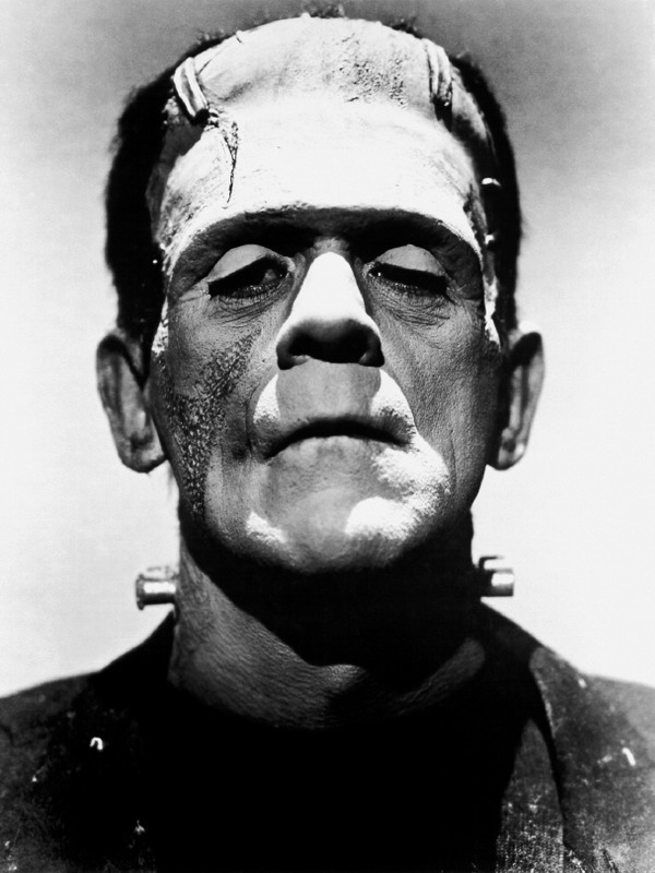
A grayscale image is simply a matrix where darkness of pixel located in coordinates (i, j) is represented by the value of its corresponding element of the matrix: a grayscale image is a dataset. This is a Voronoi diagraman of Frankenstein:

To do it I followed the next steps:

  1. Read this image
  2. Convert it to gray scale
  3. Turn it into a pure black and white image
  4. Obtain a random sample of black pixels (previous image corresponds to a sample of 6.000 points)
  5. Computes the Voronoi tesselation

Steps 1 to 3 were done with imager, a very appealing package to proccess and analice images. Step 5 was done with deldir, also a convenient package which computes Delaunay triangulation and the Dirichlet or Voronoi tessellations.

The next grid shows tesselations for sample size from 500 to 12.000 points and step equal to 500:

I gathered all previous images in this gif created with magick, another amazing package of R I discovered recently:

This is the code:

library(imager)
library(dplyr)
library(deldir)
library(ggplot2)
library(scales)

# Download the image
file="http://ereaderbackgrounds.com/movies/bw/Frankenstein.jpg"
download.file(file, destfile = "frankenstein.jpg", mode = 'wb')

# Read and convert to grayscale
load.image("frankenstein.jpg") %>% grayscale() -> x

# This is just to define frame limits
x %>% 
  as.data.frame() %>% 
  group_by() %>% 
  summarize(xmin=min(x), xmax=max(x), ymin=min(y), ymax=max(y)) %>% 
  as.vector()->rw

# Filter image to convert it to bw
x %>%
  threshold("45%") %>% 
  as.cimg() %>% 
  as.data.frame() -> df

# Function to compute and plot Voronoi tesselation depending on sample size
doPlot = function(n)
{
  #Voronoi tesselation
  df %>% 
  sample_n(n, weight=(1-value)) %>% 
  select(x,y) %>% 
  deldir(rw=rw, sort=TRUE) %>% 
  .$dirsgs -> data

  # This is just to add some alpha to lines depending on its longitude
  data %>% 
    mutate(long=sqrt((x1-x2)^2+(y1-y2)^2),
         alpha=findInterval(long, quantile(long, probs = seq(0, 1, length.out = 20)))/21)-> data

  # A little bit of ggplot to plot results
  data %>% 
    ggplot(aes(alpha=(1-alpha))) +
    geom_segment(aes(x = x1, y = y1, xend = x2, yend = y2), color="black", lwd=1) +
    scale_x_continuous(expand=c(0,0))+
    scale_y_continuous(expand=c(0,0), trans=reverse_trans())+
    theme(legend.position  = "none",
            panel.background = element_rect(fill="white"),
            axis.ticks       = element_blank(),
            panel.grid       = element_blank(),
            axis.title       = element_blank(),
            axis.text        = element_blank())->plot

return(plot)
}

# I call the previous function and store resulting plot in jpeg format
i=5000
name=paste0("frankie",i,".jpeg")
jpeg(name, width = 600, height = 800, units = "px", quality = 100)
doPlot(i)
dev.off()

# Once all images are stored I can create gif
library(magick)
frames=c()
images=list.files(pattern="jpeg")

for (i in length(images):1)
{
  x=image_read(images[i])
  x=image_scale(x, "300")
  c(x, frames) -> frames
}
animation=image_animate(frames, fps = 2)
image_write(animation, "Frankenstein.gif")