Tag Archives: complex

Playing With Julia (Set)

Viento, me pongo en movimiento y hago crecer las olas del mar que tienes dentro (Tercer Movimiento: Lo de Dentro, Extremoduro)

I really enjoy drawing complex numbers: it is a huge source of entertainment for me. In this experiment I play with the Julia Set, another beautiful fractal like this one. This is what I have done:

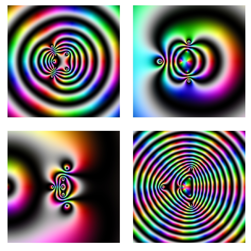
  • Choosing the function f(z)=exp(z3)-0.621
  • Generating a grid of complex numbers with both real and imaginary parts in [-2, 2]
  • Iterating f(z) over the grid a number of times so zn+1 = f(zn)
  • Drawing the resulting grid as I did here
  • Gathering all plots into a GIF with ImageMagick as I did in my previous post: each frame corresponds to a different number of iterations

This is the result:

julia

I love how easy is doing difficult things in R. You can play with the code changing f(z) as well as color palettes. Be ready to get surprised:

library(ggplot2)
library(dplyr)
library(RColorBrewer)
setwd("YOUR WORKING DIRECTORY HERE")
dir.create("output")
setwd("output")
f = function(z,c) exp(z^3)+c
# Grid of complex
z0 <- outer(seq(-2, 2, length.out = 1200),1i*seq(-2, 2, length.out = 1200),'+') %>% c()
opt <-  theme(legend.position="none",
              panel.background = element_rect(fill="white"),
              plot.margin=grid::unit(c(1,1,0,0), "mm"),
              panel.grid=element_blank(),
              axis.ticks=element_blank(),
              axis.title=element_blank(),
              axis.text=element_blank())
for (i in 1:35)
{
  z=z0
  # i iterations of f(z)
  for (k in 1:i) z <- f(z, c=-0.621) df=data.frame(x=Re(z0), y=Im(z0), z=as.vector(exp(-Mod(z)))) %>% na.omit() 
  p=ggplot(df, aes(x=x, y=y, color=z)) + 
    geom_tile() + 
    scale_x_continuous(expand=c(0,0))+
    scale_y_continuous(expand=c(0,0))+
    scale_colour_gradientn(colours=brewer.pal(8, "Paired")) + opt
  ggsave(plot=p, file=paste0("plot", stringr::str_pad(i, 4, pad = "0"),".png"), width = 1.2, height = 1.2)
}
# Place the exact path where ImageMagick is installed
system('"C:\\Program Files\\ImageMagick-6.9.3-Q16\\convert.exe" -delay 20 -loop 0 *.png julia.gif')
# cleaning up
file.remove(list.files(pattern=".png"))

Zooming

You don’t have to be beautiful to turn me on (Kiss, Prince)

I discovered recently how easy is to create GIFs with R using ImageMagick and I feel like a kid with a new toy. To begin this new era of my life as R programmer I have done this:

zooming
First of all, read this article: it explains very well how to start doing GIFs from scratch. The one I have done is inspired in this previous post where I take a set of complex numbers to transform and color it using HSV technique. In this case I use this next transformation: f(z)= -Im(z)+(Re(z)+0.5*Im(z))*1i

Modifying the range of Real and Imaginary parts of complex numbers I obtain the zooming  effect. The code is very simple. Play with it changing the transformation or the animation options. Send me your creations, I would love to see them:

library(dplyr)
library(ggplot2)
dir.create("output")
setwd("output")
id=1 # label tO name plots
for (i in seq(from=320, to=20, length.out = 38)){
z=outer(seq(from = -i, to = i, length.out = 300),1i*seq(from = -i, to = i, length.out = 500),'+') %>% c()
z0=z
for (k in 1:100) z <- -Im(z)+(Re(z)+0.5*Im(z))*1i
df=data.frame(x=Re(z0),
y=Im(z0),
h=(Arg(z)<0)*1+Arg(z)/(2*pi), s=(1+sin(2*pi*log(1+Mod(z))))/2, v=(1+cos(2*pi*log(1+Mod(z))))/2) %>% mutate(col=hsv(h,s,v))
ggplot(df, aes(x, y)) +
geom_tile(fill=df$col)+
scale_x_continuous(expand=c(0,0))+
scale_y_continuous(expand=c(0,0))+
labs(x=NULL, y=NULL)+
theme(legend.position="none",
panel.background = element_rect(fill="white"),
plot.margin=grid::unit(c(1,1,0,0), "mm"),
panel.grid=element_blank(),
axis.ticks=element_blank(),
axis.title=element_blank(),
axis.text=element_blank())
ggsave(file=paste0("plot",stringr::str_pad(id, 4, pad = "0"),".png"), width = 1, height = 1)
id=id+1
}
system('"C:\\Program Files\\ImageMagick-6.9.3-Q16\\convert.exe" -delay 10 -loop 0 -duplicate 1,-2-1 *.png zooming.gif')
# cleaning up
file.remove(list.files(pattern=".png"))

Visual Complexity

Oh, can it be, the voices calling me, they get lost and out of time (Little Black Submarines, The Black Keys)

Last October I did this experiment about complex domain coloring. Since I like giving my posts a touch of randomness, I have done this experiment. I plot four random functions on the form p1(x)*p2(x)/p3(x) where pi(x) are polynomials up-to-4th-grade with random coefficients following a chi-square distribution with degrees of freedom between 2 and 5. I measure the function over the complex plane and arrange the four resulting plots into a 2×2 grid. This is an example of the output:
Surrealism Every time you run the code you will obtain a completely different output. I have run it hundreds of times because results are always surprising. Do you want to try? Do not hesitate to send me your creations. What if you change the form of the functions or the distribution of coefficients? You can find my email here.

setwd("YOUR WORKING DIRECTORY HERE")
require(polynom)
require(ggplot2)
library(gridExtra)
ncol=2
for (i in 1:(10*ncol)) {eval(parse(text=paste("p",formatC(i, width=3, flag="0"),"=as.function(polynomial(rchisq(n=sample(2:5,1), df=sample(2:5,1))))",sep="")))}
z=as.vector(outer(seq(-5, 5, by =.02),1i*seq(-5, 5, by =.02),'+'))
opt=theme(legend.position="none",
          panel.background = element_blank(),
          panel.margin = unit(0,"null"),
          panel.grid = element_blank(),
          axis.ticks= element_blank(),
          axis.title= element_blank(),
          axis.text = element_blank(),
          strip.text =element_blank(),
          axis.ticks.length = unit(0,"null"),
          axis.ticks.margin = unit(0,"null"),
          plot.margin = rep(unit(0,"null"),4))
for (i in 1:(ncol^2))
{
  pols=sample(1:(10*ncol), 3, replace=FALSE)
  p1=paste("p", formatC(pols[1], width=3, flag="0"), "(x)*", sep="")
  p2=paste("p", formatC(pols[2], width=3, flag="0"), "(x)/", sep="")
  p3=paste("p", formatC(pols[3], width=3, flag="0"), "(x)",  sep="")
  eval(parse(text=paste("p = function (x) ", p1, p2, p3, sep="")))
  df=data.frame(x=Re(z),
                y=Im(z),
                h=(Arg(p(z))<0)*1+Arg(p(z))/(2*pi),
                s=(1+sin(2*pi*log(1+Mod(p(z)))))/2,
                v=(1+cos(2*pi*log(1+Mod(p(z)))))/2)
  g=ggplot(data=df[is.finite(apply(df,1,sum)),], aes(x=x, y=y)) + geom_tile(fill=hsv(df$h,df$s,df$v))+ opt
  assign(paste("hsv_g", formatC(i, width=3, flag="0"), sep=""), g)
}
jpeg(filename = "Surrealism.jpg", width = 800, height = 800, quality = 100)
grid.arrange(hsv_g001, hsv_g002, hsv_g003, hsv_g004, ncol=ncol)
dev.off()