Category Archives: Fractals

The Chaos Game: an experiment about fractals, recursivity and creative coding

Mathematics, rightly viewed, possesses not only truth, but supreme beauty (Bertrand Russell)

You have a pentagon defined by its five vertex. Now, follow these steps:

  • Step 0: take a point inside the pentagon (it can be its center if you want to do it easy). Keep this point in a safe place.
  • Step 1: choose a vertex randomly and take the midpoint between both of them (the vertex and the original point). Keep also this new point. Repeat Step 1 one more time.
  • Step 2: compare the last two vertex that you have chosen. If they are the same, choose another with this condition: if it’s not a neighbor of the last vertex you chose, keep it. If it is a neighbor, choose another vertex randomly until you choose a not-neighbor one. Then, take the midpoint between the last point you obtained and this new vertex. Keep also this new point.
  • Step 3: Repeat Step 2 a number of times and after that, do a plot with the set of points that you obtained.

If you repeat these steps 10 milion times, you will obtain this stunning image:

I love the incredible ability of maths to create beauty. More concretely, I love the fact of how repeating extremely simple operations can bring you to unexpected places. Would you expect that the image created with the initial naive algorithm would be that? I wouldn’t. Even knowing the result I cannot imagine how those simple steps can produce it.

The image generated by all the points repeat itself at different scales. This characteristic, called self-similarity, is property of fractals and make them extremely attractive. Step 2 is the key one to define the shape of the image. Apart of comparing two previous vertex as it’s defined in the algorithm above, I implemented two other versions:

  • one version where the currently chosen vertex cannot be the same as the previously chosen vertex.
  • another one where the currently chosen vertex cannot neighbor the previously chosen vertex if the three previously chosen vertices are the same (note that this implementation is the same as the original but comparing with three previous vertex instead two).

These images are the result of applying the three versions of the algorithm to a square, a pentagon, a hexagon and a heptagon (a row for each polygon and a column for each algorithm):

From a technical point of view I used Rcppto generate the set of points. Since each iteration depends on the previous one, the loop cannot easily vectorised and C++ is a perfect option to avoid the bottleneck if you use another technique to iterate. In this case, instead of writing the C++ directly inside the R file with cppFunction(), I used a stand-alone C++ file called chaos_funcs.cpp to write the C++ code that I load into R using sourceCpp().

Some days ago, I gave a tutorial at the coding club of the University Carlos III in Madrid where we worked with the integration of C++ and R to create beautiful images of strange attractors. The tutorial and the code we developed is here. You can also find the code of this experiment here. Enjoy!

Flowers for Julia

No hables de futuro, es una ilusión cuando el Rock & Roll conquistó mi corazón (El Rompeolas, Loquillo y los Trogloditas)

In this post I create flowers inspired in the Julia Sets, a family of fractal sets obtained from complex numbers, after being iterated by a holomorphic function. Despite of the ugly previous definition, the mechanism to create them is quite simple:

  • Take a grid of complex numbers between -2 and 2 (both, real and imaginary parts).
  • Take a function of the form  f(z)=z^{n}+c setting parameters n and c.
  • Iterate the function over the complex numbers several times. In other words: apply the function on each complex. Apply it again on the output and repeat this process a number of times.
  • Calculate the modulus of the resulting number.
  • Represent the initial complex number in a scatter plot where x-axis correspond to the real part and y-axis to the imaginary one. Color the point depending on the modulus of the resulting number after applying the function f(z) iteratively.

This image corresponds to a grid of 9 million points and 7 iterations of the function f(z)=z^{5}+0.364716021116823:

To color the points, I pick a random palette from the top list of COLOURLovers site using the colourlovers package. Since each flower involves a huge amount of calculations, I use Reduce to make this process efficiently. More examples:

There are two little Julias in the world whom I would like to dedicate this post. I wish them all the best of the world and I am sure they will discover the beauty of mathematics. These flowers are yours.

The code is available here.

Mandalas

Mathematics is a place where you can do things which you can’t do in the real world (Marcus Du Sautoy, mathematician)

From time to time I have a look to some of my previous posts: it’s like seeing them through another’s eyes. One of my first posts was this one, where I draw fractals using the Multiple Reduction Copy Machine (MRCM) algorithm. That time I was not clever enough to write an efficient code able generate deep fractals. Now I am pretty sure I could do it using ggplot and I started to do it when I come across with the idea of mixing this kind of fractal patterns with Voronoi tessellations, that I have explored in some of my previous posts, like this one. Mixing both techniques, the mandalas appeared.

I will not explain in depth the mathematics behind this patterns. I will just give a brief explanation:

  • I start obtaining n equidistant points in a unit circle centered in (0,0)
  • I repeat the process with all these points, obtaining again n points around each of them; the radius is scaled by a factor
  • I discard the previous (parent) n points

I repeat these steps iteratively. If I start with n points and iterate k times, at the end I obtain nk points. After that, I calculate the Voronoi tesselation of them, which I represent with ggplot.

This is an example:

Some others:

You can find the code here. Enjoy it.

A Shiny App to Draw Curves Based on L-System

Don’t worry about a thing ’cause every little thing gonna be alright (Three Little Birds, Bob Marley)

One of my favourite books is The Computational Beauty of Nature by Gary William Flake where there is a fantastic chapter about fractals in which I discovered the L-Systems.

L-Systems were conceived  in 1968 by Aristide Lindenmayer, a Hungarian biologist, as a mathematical description of plant growth. Apart from the Wikipedia, there are many places on the Internet where you can read about them. If you are interested, don’t miss The Algorithmic Beauty of Plants, an awesome book by Przemysław Prusinkiewicz that you can obtain here for free.

Roughly speaking, a L-System is a very efficient way to make drawings. In its simplest way consists in two different actions: draw a straigh line and change the angle. This is just what you need, for example, to draw a square: draw a straigh line of  any length, turn 90 degrees (without drawing), draw another straigh line of the same length, turn 90 degrees in the same direction, draw, turn and draw again. Denoting F as the action of drawing a line of length d and + as turning 90 degrees right, the whole process to draw a square can be represented as F+F+F+F.

L-Systems are quite simple to program in R. You only need to substitute the rules iteratively into the axiom (I use gsubfn function to do it) and split the resulting chain into parts with str_extract_all, for example. The result is a set of very simple actions (draw or turn) that can be visualized with ggplot and its path geometry. There are four important parameters in L-Systems:

  • The seed of the drawing, called axiom
  • The substitutions to be applied iteratively, called rules
  • How many times to apply substitutions, called depth
  • Angle of each turning

For example, let’s define the next L-System:

  • Axiom: F-F-F-F
  • Rule: F → F−F+F+FF−F−F+F

The rule means that every F must be replaced by F−F+F+FF−F−F+F while + means right turning and - left one. After one iteration, the axiom is replaced by F-F+F+FF-F-F+F-F-F+F+FF-F-F+F-F-F+F+FF-F-F+F-F-F+F+FF-F-F+F and iterating again, the new string is F-F+F+FF-F-F+F-F-F+F+FF-F-F+F+F-F+F+FF-F-F+F+F-F+F+FF-F-F+FF-F+F+FF-F-F+F-F-F+F+FF-F-F+F-F-F+F+FF-F-F+F+F-F+F+FF-F-F+F-F-F+F+FF-F-F+F-F-F+F+FF-F-F+F+F-F+F+FF-F-F+F+F-F+F+FF-F-F+FF-F+F+FF-F-F+F-F-F+F+FF-F-F+F-F-F+F+FF-F-F+F+F-F+F+FF-F-F+F-F-F+F+FF-F-F+F-F-F+F+FF-F-F+F+F-F+F+FF-F-F+F+F-F+F+FF-F-F+FF-F+F+FF-F-F+F-F-F+F+FF-F-F+F-F-F+F+FF-F-F+F+F-F+F+FF-F-F+F-F-F+F+FF-F-F+F-F-F+F+FF-F-F+F+F-F+F+FF-F-F+F+F-F+F+FF-F-F+FF-F+F+FF-F-F+F-F-F+F+FF-F-F+F-F-F+F+FF-F-F+F+F-F+F+FF-F-F+F. As you can see, the length of the string grows exponentially. Converting last string into actions, produces this drawing, called Koch Island:

It is funny how different axioms and rules produce very different drawings. I have done a Shiny App to play with L-systems. Although it is quite simple, it has two interesting features I would like to undeline:

  • Delay reactions with eventReactive to allow to set depth and angle values before refreshing the plot
  • Build a dynamic UI that reacts to user input depending on the curve choosen

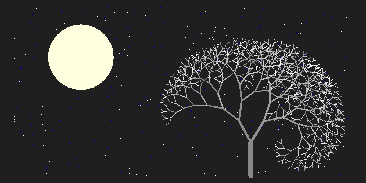
There are twelve curves in the application: Koch Island (and 6 variations), cuadratic snowflake, Sierpinsky triangle, hexagonal Gosper, quadratic Gosper and Dragon curve. These are their plots:

The definition of all these curves (axiom and rules) can be found in the first chapter of the Prusinkiewicz’s book. The magic comes when you modify angles and colors. These are some examples among the infinite number of possibilities that can be created:

I enjoyed a lot doing and playing with the app. You can try it here. If you do a nice drawing, please let me know in Twitter or dropping me an email. This is the code of the App:

ui.R:

library(shiny)

shinyUI(fluidPage(
  titlePanel("Curves based on L-systems"),
  
  sidebarLayout(
    sidebarPanel(
      selectInput("cur", "Choose a curve:",
                  c("","Koch Island",
                    "Cuadratic Snowflake",
                    "Koch Variation 1",
                    "Koch Variation 2",
                    "Koch Variation 3",
                    "Koch Variation 4",
                    "Koch Variation 5",
                    "Koch Variation 6",
                    "Sierpinsky Triangle",
                    "Dragon Curve",
                    "Hexagonal Gosper Curve",
                    "Quadratic Gosper Curve"),
                  selected = ""),
      
      conditionalPanel(
        condition = "input.cur != \"\"",
        uiOutput("Iterations")),
      
      conditionalPanel(
        condition = "input.cur != \"\"",
        uiOutput("Angle")),
      
      conditionalPanel(
        condition = "input.cur != \"\"",
        selectInput("lic", label = "Line color:", choices = colors(), selected = "black")),
      
      
      conditionalPanel(
        condition = "input.cur != \"\"",
        selectInput("bac", label = "Background color:", choices = colors(), selected = "white")),
      
      conditionalPanel(
        condition = "input.cur != \"\"",
        actionButton(inputId = "go", label = "Go!", 
                     style="color: #fff; background-color: #337ab7; border-color: #2e6da4"))


    ), 
    mainPanel(plotOutput("curve", height="550px", width = "100%"))
  )
  
))

server.R:

library(shiny)
library(gsubfn)
library(stringr)
library(dplyr)
library(ggplot2)
library(rlist)

shinyServer(function(input, output) {
   
  curves=list(
    list(name="Koch Island",
         axiom="F-F-F-F",
         rules=list("F"="F-F+F+FF-F-F+F"),
         angle=90,
         n=2,
         alfa0=90),
    list(name="Cuadratic Snowflake",
         axiom="-F",
         rules=list("F"="F+F-F-F+F"),
         angle=90,
         n=4,
         alfa0=90),
    list(name="Koch Variation 1",
         axiom="F-F-F-F",
         rules=list("F"="FF-F-F-F-F-F+F"),
         angle=90,
         n=3,
         alfa0=90),
    list(name="Koch Variation 2",
         axiom="F-F-F-F",
         rules=list("F"="FF-F-F-F-FF"),
         angle=90,
         n=4,
         alfa0=90),
    list(name="Koch Variation 3",
         axiom="F-F-F-F",
         rules=list("F"="FF-F+F-F-FF"),
         angle=90,
         n=3,
         alfa0=90),
    list(name="Koch Variation 4",
         axiom="F-F-F-F",
         rules=list("F"="FF-F--F-F"),
         angle=90,
         n=4,
         alfa0=90),
    list(name="Koch Variation 5",
         axiom="F-F-F-F",
         rules=list("F"="F-FF--F-F"),
         angle=90,
         n=5,
         alfa0=90),
    list(name="Koch Variation 6",
         axiom="F-F-F-F",
         rules=list("F"="F-F+F-F-F"),
         angle=90,
         n=4,
         alfa0=90),
    list(name="Sierpinsky Triangle",
         axiom="R",
         rules=list("L"="R+L+R", "R"="L-R-L"),
         angle=60,
         n=6,
         alfa0=0),
    list(name="Dragon Curve",
         axiom="L",
         rules=list("L"="L+R+", "R"="-L-R"),
         angle=90,
         n=10,
         alfa0=90),
    list(name="Hexagonal Gosper Curve",
         axiom="L",
         rules=list("L"="L+R++R-L--LL-R+", "R"="-L+RR++R+L--L-R"),
         angle=60,
         n=4,
         alfa0=60),
    list(name="Quadratic Gosper Curve",
         axiom="-R",
         rules=list("L"="LL-R-R+L+L-R-RL+R+LLR-L+R+LL+R-LR-R-L+L+RR-", 
                    "R"="+LL-R-R+L+LR+L-RR-L-R+LRR-L-RL+L+R-R-L+L+RR"),
         angle=90,
         n=2,
         alfa0=90))
  
  output$Iterations <- renderUI({ if (input$cur!="") curve=list.filter(curves, name==input$cur) else curve=list.filter(curves, name=="Koch Island") iterations=list.select(curve, n) %>% unlist
    numericInput("ite", "Depth:", iterations, min = 1, max = (iterations+2))
  })
  
  output$Angle <- renderUI({ curve=list.filter(curves, name==input$cur) angle=list.select(curve, angle) %>% unlist
    numericInput("ang", "Angle:", angle, min = 0, max = 360)
  })
  
  data <- eventReactive(input$go, { curve=list.filter(curves, name==input$cur) axiom=list.select(curve, axiom) %>% unlist
    rules=list.select(curve, rules)[[1]]$rules
    alfa0=list.select(curve, alfa0) %>% unlist
    
    for (i in 1:input$ite) axiom=gsubfn(".", rules, axiom)
    actions=str_extract_all(axiom, "\\d*\\+|\\d*\\-|F|L|R|\\[|\\]|\\|") %>% unlist
    
    points=data.frame(x=0, y=0, alfa=alfa0)
    for (i in 1:length(actions)) 
    {
      if (actions[i]=="F"|actions[i]=="L"|actions[i]=="R")
      {
        x=points[nrow(points), "x"]+cos(points[nrow(points), "alfa"]*(pi/180))
        y=points[nrow(points), "y"]+sin(points[nrow(points), "alfa"]*(pi/180))
        alfa=points[nrow(points), "alfa"]
        points %>% rbind(data.frame(x=x, y=y, alfa=alfa)) -> points
      }
      else{
        alfa=points[nrow(points), "alfa"]
        points[nrow(points), "alfa"]=eval(parse(text=paste0("alfa",actions[i], input$ang)))
      }
    }
    return(points)
  })
  
  output$curve <- renderPlot({    
    ggplot(data(), aes(x, y)) + 
      geom_path(color=input$lic) + 
      coord_fixed(ratio = 1) +
      theme(legend.position="none",
            panel.background = element_rect(fill=input$bac),
            panel.grid=element_blank(),
            axis.ticks=element_blank(),
            axis.title=element_blank(),
            axis.text=element_blank())
  })
    
})

Playing With Julia (Set)

Viento, me pongo en movimiento y hago crecer las olas del mar que tienes dentro (Tercer Movimiento: Lo de Dentro, Extremoduro)

I really enjoy drawing complex numbers: it is a huge source of entertainment for me. In this experiment I play with the Julia Set, another beautiful fractal like this one. This is what I have done:

  • Choosing the function f(z)=exp(z3)-0.621
  • Generating a grid of complex numbers with both real and imaginary parts in [-2, 2]
  • Iterating f(z) over the grid a number of times so zn+1 = f(zn)
  • Drawing the resulting grid as I did here
  • Gathering all plots into a GIF with ImageMagick as I did in my previous post: each frame corresponds to a different number of iterations

This is the result:

julia

I love how easy is doing difficult things in R. You can play with the code changing f(z) as well as color palettes. Be ready to get surprised:

library(ggplot2)
library(dplyr)
library(RColorBrewer)
setwd("YOUR WORKING DIRECTORY HERE")
dir.create("output")
setwd("output")
f = function(z,c) exp(z^3)+c
# Grid of complex
z0 <- outer(seq(-2, 2, length.out = 1200),1i*seq(-2, 2, length.out = 1200),'+') %>% c()
opt <-  theme(legend.position="none",
              panel.background = element_rect(fill="white"),
              plot.margin=grid::unit(c(1,1,0,0), "mm"),
              panel.grid=element_blank(),
              axis.ticks=element_blank(),
              axis.title=element_blank(),
              axis.text=element_blank())
for (i in 1:35)
{
  z=z0
  # i iterations of f(z)
  for (k in 1:i) z <- f(z, c=-0.621) df=data.frame(x=Re(z0), y=Im(z0), z=as.vector(exp(-Mod(z)))) %>% na.omit() 
  p=ggplot(df, aes(x=x, y=y, color=z)) + 
    geom_tile() + 
    scale_x_continuous(expand=c(0,0))+
    scale_y_continuous(expand=c(0,0))+
    scale_colour_gradientn(colours=brewer.pal(8, "Paired")) + opt
  ggsave(plot=p, file=paste0("plot", stringr::str_pad(i, 4, pad = "0"),".png"), width = 1.2, height = 1.2)
}
# Place the exact path where ImageMagick is installed
system('"C:\\Program Files\\ImageMagick-6.9.3-Q16\\convert.exe" -delay 20 -loop 0 *.png julia.gif')
# cleaning up
file.remove(list.files(pattern=".png"))

Going Bananas With Hilbert

It seemed that everything is in ruins, and that all the basic mathematical concepts have lost their meaning (Naum Vilenkin, Russian mathematician, regarding to the discovery of Peano’s curve)

Giuseppe Peano found in 1890 a way to draw a curve in the plane that filled the entire space: just a simple line covering completely a two dimensional plane. Its discovery meant a big earthquake in the traditional structure of mathematics. Peano’s curve was the first but not the last: one of these space-filling curves was discovered by Hilbert and takes his name. It is really beautiful:
hilbert_n5

Hilbert’s curve can be created iteratively. These are the first six iterations of its construction:
hilbert

As you will see below, R code to create Hilbert’s curve is extremely easy. It is also very easy to play with the curve, altering the order in which points are sorted. Changing the initial matrix(1) by some other number, resulting curves are quite appealing:

Let’s go futher. Changing ggplot geometry from geom_path to geom_polygon generate some crazy pseudo-tessellations:

And what if you change the matrix exponent?

And what if you apply polar coordinates?

We started with a simple line and with some small changes we have created fantastical images. And all these things only using black and white. Do you want to add some colors? Try with the following code (if you draw something interesting, please let me know):

library(reshape2)
library(dplyr)
library(ggplot2)
opt=theme(legend.position="none",
          panel.background = element_rect(fill="white"),
          panel.grid=element_blank(),
          axis.ticks=element_blank(),
          axis.title=element_blank(),
          axis.text=element_blank())
hilbert = function(m,n,r) {
  for (i in 1:n)
  {
    tmp=cbind(t(m), m+nrow(m)^2)
    m=rbind(tmp, (2*nrow(m))^r-tmp[nrow(m):1,]+1)
  }
  melt(m) %>% plyr::rename(c("Var1" = "x", "Var2" = "y", "value"="order")) %>% arrange(order)}
# Original
ggplot(hilbert(m=matrix(1), n=1, r=2), aes(x, y)) + geom_path()+ opt
ggplot(hilbert(m=matrix(1), n=2, r=2), aes(x, y)) + geom_path()+ opt
ggplot(hilbert(m=matrix(1), n=3, r=2), aes(x, y)) + geom_path()+ opt
ggplot(hilbert(m=matrix(1), n=4, r=2), aes(x, y)) + geom_path()+ opt
ggplot(hilbert(m=matrix(1), n=5, r=2), aes(x, y)) + geom_path()+ opt
ggplot(hilbert(m=matrix(1), n=6, r=2), aes(x, y)) + geom_path()+ opt
# Changing order
ggplot(hilbert(m=matrix(.5), n=5, r=2), aes(x, y)) + geom_path()+ opt
ggplot(hilbert(m=matrix(0), n=5, r=2), aes(x, y)) + geom_path()+ opt
ggplot(hilbert(m=matrix(tan(1)), n=5, r=2), aes(x, y)) + geom_path()+ opt
ggplot(hilbert(m=matrix(3), n=5, r=2), aes(x, y)) + geom_path()+ opt
ggplot(hilbert(m=matrix(-1), n=5, r=2), aes(x, y)) + geom_path()+ opt
ggplot(hilbert(m=matrix(log(.1)), n=5, r=2), aes(x, y)) + geom_path()+ opt
ggplot(hilbert(m=matrix(-15), n=5, r=2), aes(x, y)) + geom_path()+ opt
ggplot(hilbert(m=matrix(-0.001), n=5, r=2), aes(x, y)) + geom_path()+ opt
# Polygons
ggplot(hilbert(m=matrix(log(1)), n=4, r=2), aes(x, y)) + geom_polygon()+ opt
ggplot(hilbert(m=matrix(.5), n=4, r=2), aes(x, y)) + geom_polygon()+ opt
ggplot(hilbert(m=matrix(tan(1)), n=5, r=2), aes(x, y)) + geom_polygon()+ opt
ggplot(hilbert(m=matrix(-15), n=4, r=2), aes(x, y)) + geom_polygon()+ opt
ggplot(hilbert(m=matrix(-25), n=4, r=2), aes(x, y)) + geom_polygon()+ opt
ggplot(hilbert(m=matrix(0), n=4, r=2), aes(x, y)) + geom_polygon()+ opt
ggplot(hilbert(m=matrix(1000000), n=4, r=2), aes(x, y)) + geom_polygon()+ opt
ggplot(hilbert(m=matrix(-1), n=4, r=2), aes(x, y)) + geom_polygon()+ opt
ggplot(hilbert(m=matrix(-.00001), n=4, r=2), aes(x, y)) + geom_polygon()+ opt
# Changing exponent
gplot(hilbert(m=matrix(log(1)), n=4, r=-1), aes(x, y)) + geom_polygon()+ opt
ggplot(hilbert(m=matrix(.5), n=4, r=-2), aes(x, y)) + geom_polygon()+ opt
ggplot(hilbert(m=matrix(tan(1)), n=4, r=6), aes(x, y)) + geom_polygon()+ opt
ggplot(hilbert(m=matrix(-15), n=3, r=sin(2)), aes(x, y)) + geom_polygon()+ opt
ggplot(hilbert(m=matrix(-25), n=4, r=-.0001), aes(x, y)) + geom_polygon()+ opt
ggplot(hilbert(m=matrix(0), n=4, r=200), aes(x, y)) + geom_polygon()+ opt
ggplot(hilbert(m=matrix(1000000), n=3, r=.5), aes(x, y)) + geom_polygon()+ opt
ggplot(hilbert(m=matrix(-1), n=4, r=sqrt(2)), aes(x, y)) + geom_polygon()+ opt
ggplot(hilbert(m=matrix(-.00001), n=4, r=52), aes(x, y)) + geom_polygon()+ opt
# Polar coordinates
ggplot(hilbert(m=matrix(1), n=4, r=2), aes(x, y)) + geom_polygon()+ coord_polar()+opt
ggplot(hilbert(m=matrix(-1), n=5, r=2), aes(x, y)) + geom_polygon()+ coord_polar()+opt
ggplot(hilbert(m=matrix(.1), n=2, r=.5), aes(x, y)) + geom_polygon()+ coord_polar()+opt
ggplot(hilbert(m=matrix(1000000), n=2, r=.1), aes(x, y)) + geom_polygon()+ coord_polar()+opt
ggplot(hilbert(m=matrix(.25), n=3, r=3), aes(x, y)) + geom_polygon()+ coord_polar()+opt
ggplot(hilbert(m=matrix(tan(1)), n=5, r=1), aes(x, y)) + geom_polygon()+ coord_polar()+opt
ggplot(hilbert(m=matrix(1), n=4, r=1), aes(x, y)) + geom_polygon()+ coord_polar()+opt
ggplot(hilbert(m=matrix(log(1)), n=3, r=sin(2)), aes(x, y)) + geom_polygon()+ coord_polar()+opt
ggplot(hilbert(m=matrix(-.0001), n=4, r=25), aes(x, y)) + geom_polygon()+ coord_polar()+opt

The Pythagorean Tree Is In Bloom

There is geometry in the humming of the strings, there is music in the spacing of the spheres (Pythagoras)

Spring is here and I will be on holiday next week. I cannot be more happy! It is time to celebrate so I have drawn another fractal. It is called the Pythagorean Tree:

PythagoreanTree

Here you have the code. See you soon:

library("grid")
l=0.15 #Length of the square
grid.newpage()
gr <- rectGrob(width=l, height=l, name="gr") #Basic Square
pts <- data.frame(level=1, x=0.5, y=0.1, alfa=0) #Centers of the squares
for (i in 2:10) #10=Deep of the fractal. Feel free to change it
{
  df<-pts[pts$level==i-1,]
  for (j in 1:nrow(df))
  {
    pts <- rbind(pts, 
                 c(i, 
                   df[j,]$x-2*l*((1/sqrt(2))^(i-1))*sin(df[j,]$alfa+pi/4)-0.5*l*((1/sqrt(2))^(i-2))*sin(df[j,]$alfa+pi/4-3*pi/4), 
                   df[j,]$y+2*l*((1/sqrt(2))^(i-1))*cos(df[j,]$alfa+pi/4)+0.5*l*((1/sqrt(2))^(i-2))*cos(df[j,]$alfa+pi/4-3*pi/4),                  
                   df[j,]$alfa+pi/4))
    pts <- rbind(pts, 
                 c(i, 
                   df[j,]$x-2*l*((1/sqrt(2))^(i-1))*sin(df[j,]$alfa-pi/4)-0.5*l*((1/sqrt(2))^(i-2))*sin(df[j,]$alfa-pi/4+3*pi/4), 
                   df[j,]$y+2*l*((1/sqrt(2))^(i-1))*cos(df[j,]$alfa-pi/4)+0.5*l*((1/sqrt(2))^(i-2))*cos(df[j,]$alfa-pi/4+3*pi/4),                  
                   df[j,]$alfa-pi/4))
  }
}
for (i in 1:nrow(pts))
{
  grid.draw(editGrob(gr, vp=viewport(x=pts[i,]$x, y=pts[i,]$y, w=((1/sqrt(2))^(pts[i,]$level-1)), h=((1/sqrt(2))^(pts[i,]$level-1)), angle=pts[i,]$alfa*180/pi), 
            gp=gpar(col=0, lty="solid", fill=rgb(139*(nrow(pts)-i)/(nrow(pts)-1), 
                                                 (186*i+69*nrow(pts)-255)/(nrow(pts)-1), 
                                                  19*(nrow(pts)-i)/(nrow(pts)-1), 
                                                  alpha= (-110*i+200*nrow(pts)-90)/(nrow(pts)-1), max=255))))
}

The Collatz Fractal

It seems to me that the poet has only to perceive that which others do not perceive, to look deeper than others look. And the mathematician must do the same thing (Sofia Kovalevskaya)

How beautiful is this fractal! In previous posts I colored plots using module of complex numbers generated after some iterations. In this occasion I have used the escape-time algorithm, a very well known coloring algorithm which is very easy to implement in R.
Collatz07
Those who want to know more about this fractal can go here. For coloring, I chose a simple scale from red to yellow resulting a fractal interpretation of my country’s flag. You can choose another scale or use a RColorBrewer palette as I did in this previous post. Choosing another x or y ranges you can zoom particular areas of the fractal.

Try yourself and send me your pictures!

library(ggplot2)
xrange <- seq(-8, 8, by = 0.01)
yrange <- seq(-3, 3, by = 0.01)
f  <- function (z) {1/4*(2+7*z-(2+5*z)*cos(pi*z))}
z <- outer(xrange, 1i*yrange,'+')
t <- mat.or.vec(nrow(z), ncol(z))
for (k in 1:10)
{
  z <- f(z)
  t <- t + (is.finite(z)+0)
}
## Supressing texts, titles, ticks, background and legend.
opt <- theme(legend.position="none",
             panel.background = element_blank(),
             axis.ticks=element_blank(),
             axis.title=element_blank(),
             axis.text =element_blank())
z <- data.frame(expand.grid(x=xrange, y=yrange), z=as.vector(t))
ggplot(z, aes(x=x, y=y, color=z)) + geom_tile() + scale_colour_gradient(low="red", high="yellow") + opt

Blurry Fractals

Beauty is the first test; there is no permanent place in the world for ugly mathematics (G. H. Hardy)

Newton basin fractals are the result of iterating Newton’s method to find roots of a polynomial over the complex plane. It maybe sound a bit complicated but is actually quite simple to understand. Those who would like to read some more about Newton basin fractals can visit this page.

This fractals are very easy to generate in R and produce very nice images. Making a small number of iterations, resulting images seems to be blurred when are represented with tile geometry in ggplot. Combined with palettes provided by RColorBrewer give rise to very interesting images. Here you have some examples:

Result for f(z)=z3-1 and palette equal to Set3:Blurry1-Set3Result for f(z)=z4+z-1 and palette equal to Paired:Blurry2-PairedResult for f(z)=z5+z3+z-1 and palette equal to Dark2:Blurry3-Dark2Here you have the code. If you generate nice pictures I will be very grateful if you send them to me:

library(ggplot2)
library(numDeriv)
library(RColorBrewer)
library(gridExtra)
## Polynom: choose only one or try yourself
f  <- function (z) {z^3-1}        #Blurry 1
#f  <- function (z) {z^4+z-1}     #Blurry 2
#f  <- function (z) {z^5+z^3+z-1} #Blurry 3
z <- outer(seq(-2, 2, by = 0.01),1i*seq(-2, 2, by = 0.01),'+')
for (k in 1:5) z <- z-f(z)/matrix(grad(f, z), nrow=nrow(z))
## Supressing texts, titles, ticks, background and legend.
opt <- theme(legend.position="none",
             panel.background = element_blank(),
             axis.ticks=element_blank(), 
             axis.title=element_blank(), 
             axis.text =element_blank())
z <- data.frame(expand.grid(x=seq(ncol(z)), y=seq(nrow(z))), z=as.vector(exp(-Mod(f(z)))))
# Create plots. Choose a palette with display.brewer.all()
p1 <- ggplot(z, aes(x=x, y=y, color=z)) + geom_tile() + scale_colour_gradientn(colours=brewer.pal(8, "Paired")) + opt
p2 <- ggplot(z, aes(x=x, y=y, color=z)) + geom_tile() + scale_colour_gradientn(colours=brewer.pal(7, "Paired")) + opt
p3 <- ggplot(z, aes(x=x, y=y, color=z)) + geom_tile() + scale_colour_gradientn(colours=brewer.pal(6, "Paired")) + opt
p4 <- ggplot(z, aes(x=x, y=y, color=z)) + geom_tile() + scale_colour_gradientn(colours=brewer.pal(5, "Paired")) + opt
# Arrange four plots in a 2x2 grid
grid.arrange(p1, p2, p3, p4, ncol=2)

The Lonely Acacia Is Rocked By The Wind Of The African Night

If you can walk you can dance. If you can talk you can sing (Zimbabwe Proverb)

There are two things in this picture I would like to emphasise. First one is that everything is made using points and lines. The moon is an enormous point, stars are three small nested points and the tree is a set of straight lines. Points and lines over a simple cartesian graph, no more. Second one is that the tree is a jittered fractal. In particular, is a jittered L-system fractal, a formalism invented in 1968 by a biologist (Aristid Lindemayer) that yields a mathematical description of plan growth. Why jittered? Because I add some positive noise to the angle in which branches are divided by two iteratively. It gives to the tree the sense to be rocked by the wind. This is the picture:

image1

I generated 120 images and gathered in this video to make the wind happen. The stunning song is called Kothbiro performed by Ayub Ogada.

Here you have the code:

depth <- 9
angle<-30 #Between branches division
L <- 0.90 #Decreasing rate of branches by depth
nstars <- 300 #Number of stars to draw
mstars <- matrix(runif(2*nstars), ncol=2)
branches <- rbind(c(1,0,0,abs(jitter(0)),1,jitter(5, amount = 5)), data.frame())
colnames(branches) <- c("depth", "x1", "y1", "x2", "y2", "inertia")
for(i in 1:depth)
{
  df <- branches[branches$depth==i,]
  for(j in 1:nrow(df))
  {
    branches <- rbind(branches, c(df[j,1]+1, df[j,4], df[j,5], df[j,4]+L^(2*i+1)*sin(pi*(df[j,6]+angle)/180), df[j,5]+L^(2*i+1)*cos(pi*(df[j,6]+angle)/180), df[j,6]+angle+jitter(10, amount = 8)))
    branches <- rbind(branches, c(df[j,1]+1, df[j,4], df[j,5], df[j,4]+L^(2*i+1)*sin(pi*(df[j,6]-angle)/180), df[j,5]+L^(2*i+1)*cos(pi*(df[j,6]-angle)/180), df[j,6]-angle+jitter(10, amount = 8)))
  }
}
nodes <- rbind(as.matrix(branches[,2:3]), as.matrix(branches[,4:5]))
png("image.png", width = 1200, height = 600)
plot.new()
par(mai = rep(0, 4), bg = "gray12")
plot(nodes, type="n", xlim=c(-7, 3), ylim=c(0, 5))
for (i in 1:nrow(mstars)) 
{
  points(x=10*mstars[i,1]-7, y=5*mstars[i,2], col = "blue4", cex=.7, pch=16)
  points(x=10*mstars[i,1]-7, y=5*mstars[i,2], col = "blue",  cex=.3, pch=16)
  points(x=10*mstars[i,1]-7, y=5*mstars[i,2], col = "white", cex=.1, pch=16)
}
# The moon
points(x=-5, y=3.5, cex=40, pch=16, col="lightyellow")
# The tree
for (i in 1:nrow(branches)) {lines(x=branches[i,c(2,4)], y=branches[i,c(3,5)], col = paste("gray", as.character(sample(seq(from=50, to=round(50+5*branches[i,1]), by=1), 1)), sep = ""), lwd=(65/(1+3*branches[i,1])))}
rm(branches)
dev.off()