Tag Archives: beauty

The Lonely Acacia Is Rocked By The Wind Of The African Night

If you can walk you can dance. If you can talk you can sing (Zimbabwe Proverb)

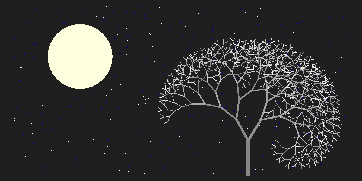
There are two things in this picture I would like to emphasise. First one is that everything is made using points and lines. The moon is an enormous point, stars are three small nested points and the tree is a set of straight lines. Points and lines over a simple cartesian graph, no more. Second one is that the tree is a jittered fractal. In particular, is a jittered L-system fractal, a formalism invented in 1968 by a biologist (Aristid Lindemayer) that yields a mathematical description of plan growth. Why jittered? Because I add some positive noise to the angle in which branches are divided by two iteratively. It gives to the tree the sense to be rocked by the wind. This is the picture:

image1

I generated 120 images and gathered in this video to make the wind happen. The stunning song is called Kothbiro performed by Ayub Ogada.

Here you have the code:

depth <- 9
angle<-30 #Between branches division
L <- 0.90 #Decreasing rate of branches by depth
nstars <- 300 #Number of stars to draw
mstars <- matrix(runif(2*nstars), ncol=2)
branches <- rbind(c(1,0,0,abs(jitter(0)),1,jitter(5, amount = 5)), data.frame())
colnames(branches) <- c("depth", "x1", "y1", "x2", "y2", "inertia")
for(i in 1:depth)
{
  df <- branches[branches$depth==i,]
  for(j in 1:nrow(df))
  {
    branches <- rbind(branches, c(df[j,1]+1, df[j,4], df[j,5], df[j,4]+L^(2*i+1)*sin(pi*(df[j,6]+angle)/180), df[j,5]+L^(2*i+1)*cos(pi*(df[j,6]+angle)/180), df[j,6]+angle+jitter(10, amount = 8)))
    branches <- rbind(branches, c(df[j,1]+1, df[j,4], df[j,5], df[j,4]+L^(2*i+1)*sin(pi*(df[j,6]-angle)/180), df[j,5]+L^(2*i+1)*cos(pi*(df[j,6]-angle)/180), df[j,6]-angle+jitter(10, amount = 8)))
  }
}
nodes <- rbind(as.matrix(branches[,2:3]), as.matrix(branches[,4:5]))
png("image.png", width = 1200, height = 600)
plot.new()
par(mai = rep(0, 4), bg = "gray12")
plot(nodes, type="n", xlim=c(-7, 3), ylim=c(0, 5))
for (i in 1:nrow(mstars)) 
{
  points(x=10*mstars[i,1]-7, y=5*mstars[i,2], col = "blue4", cex=.7, pch=16)
  points(x=10*mstars[i,1]-7, y=5*mstars[i,2], col = "blue",  cex=.3, pch=16)
  points(x=10*mstars[i,1]-7, y=5*mstars[i,2], col = "white", cex=.1, pch=16)
}
# The moon
points(x=-5, y=3.5, cex=40, pch=16, col="lightyellow")
# The tree
for (i in 1:nrow(branches)) {lines(x=branches[i,c(2,4)], y=branches[i,c(3,5)], col = paste("gray", as.character(sample(seq(from=50, to=round(50+5*branches[i,1]), by=1), 1)), sep = ""), lwd=(65/(1+3*branches[i,1])))}
rm(branches)
dev.off()

Warholing Grace With Clara

Do not believe anything: what artists really do is to hang around all day (Paco de Lucia)

Andy Warhol was mathematician. At least, he knew how clustering algorithms work. I am pretty sure of this after doing this experiment.  First of all, let me introduce you to the breathtaking Grace Kelly:

936full-grace-kelly

In my previous post I worked also with images showing how simple is to operate with them since they are represented by matrices. This is another example of this. Third dimension of an image matrix is an 3D array representing color of pixels in (r, g, b) format. Applying a cluster algorithm over this information generates groups of pixels with similar color. I used cluster package and because of the high size of picture I decided to use clara algorithm which is extremely fast. Apart of its high speed, another advantage of clara is that clusters are represented by real elements of the population, called medoids, instead of being by average individuals as k-means do. It fits very well with my purposes because once clusters are calculated I only have to change each pixel by its medoid and plot it. Setting clara to divide pixels into 2 groups, generates a 2 colored image. Setting it to 3 groups, generates a 3 colored one and so on. Following, you can find results from 2 to 7 groups:

Warholing2 Warholing3 Warholing4
Warholing5 Warholing6 Warholing7

Working with samples can be a handicap, maybe less important than the speed it produces. Sometimes images generated by n groups seems to be worse fitted than the one generated by n-1 groups. You can see it in this video, where results from 1 to 60 groups are presented sequentially. It only takes 42 seconds.

Here you have the code. Feel free to warholing:

library("biOps")
library("abind")
library("reshape")
library("reshape2")
library("cluster")
library("sp")
#######################################################################################################
#Initialization
#######################################################################################################
x     <- readJpeg("936full-grace-kelly.jpg")
plot(x)
#######################################################################################################
#Data
#######################################################################################################
data <- merge(merge(melt(x[,,1]), melt(x[,,2]), by=c("X1", "X2")), melt(x[,,3]), by=c("X1", "X2"))
colnames(data) <- c("X1", "X2", "r", "g", "b")
#######################################################################################################
#Clustering
#######################################################################################################
colors <- 5
clarax <- clara(data[,3:5], colors)
datacl   <- data.frame(data, clarax$cluster)
claradf2 <- as.data.frame(clarax$medoids)
claradf2$id <- as.numeric(rownames(claradf2))
colnames(claradf2) <- c("r", "g", "b", "clarax.cluster")
claradf <- merge(datacl, claradf2, by=c("clarax.cluster"))
colnames(claradf) <-c("clarax.cluster", "X1", "X2", "r.x", "g.x", "b.x", "r.y", "g.y", "b.y")
datac <- claradf[do.call("order", claradf[c("X1", "X2")]), ]
x1<-acast(datac[,c(2,3,7)], X1~X2, value.var="r.y") 
x2<-acast(datac[,c(2,3,8)], X1~X2, value.var="g.y") 
x3<-acast(datac[,c(2,3,9)], X1~X2, value.var="b.y") 
warhol <- do.call(abind, c(list(x1,x2,x3), along = 3))
plot(imagedata(warhol))
writeJpeg(paste("Warholing", as.character(colors), ".jpg", sep=""), imagedata(warhol))