Tag Archives: RColorBrewer

Polar Circles

You cannot find peace by avoiding life (Virginia Woolf)

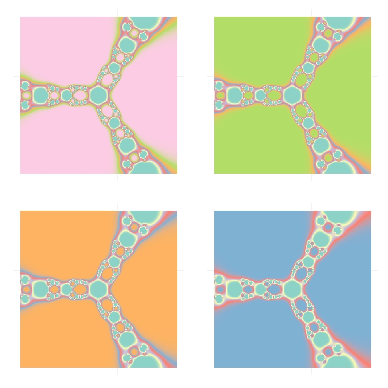
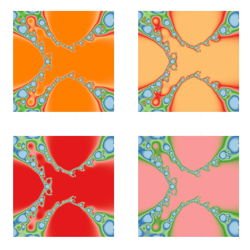
Combining polar coordinates, RColorBrewer palettes, ggplot2 and a simple trigonometric function to define the width of the tiles is easy to produce nice circular plots like these:

polar_flower4polar_flower2polar_flower1polar_flower3

Do you want to try? Here you have the code:

library(ggplot2)
library(dplyr)
library(RColorBrewer)
n=500
m=50
w=sapply(seq(from=-3.5*pi, to=3.5*pi, length.out=n), function(x) {abs(sin(x))})
x=c(1)
for (i in 2:n) {x[i]=x[i-1]+1/2*(w[i-1]+w[i])}
expand.grid(x=x, y=1:m) %>%
  mutate(w=rep(w, m))-> df
opt=theme(legend.position="none",
          panel.background = element_rect(fill="white"),
          panel.grid=element_blank(),
          axis.ticks=element_blank(),
          axis.title=element_blank(),
          axis.text=element_blank())
ggplot(df, aes(x=x,y=y))+geom_tile(aes(fill=x, width=w))+ 
  scale_fill_gradient(low=brewer.pal(9, "Greens")[1], high=brewer.pal(9, "Greens")[9])+
  coord_polar(start = runif(1, min = 0, max = 2*pi))+opt
ggplot(df, aes(x=x,y=y))+geom_tile(aes(fill=w, width=w))+ 
  scale_fill_gradient(low=brewer.pal(9, "Reds")[1], high=brewer.pal(9, "Reds")[9])+ 
  coord_polar(start = runif(1, min = 0, max = 2*pi))+opt
ggplot(df, aes(x=x,y=y))+geom_tile(aes(fill=y, width=w))+ 
  scale_fill_gradient(low=brewer.pal(9, "Purples")[1], high=brewer.pal(9, "Purples")[9])+ 
  coord_polar(start = runif(1, min = 0, max = 2*pi))+opt
ggplot(df, aes(x=x,y=y))+geom_tile(aes(fill=w*y, width=w))+ 
  scale_fill_gradient(low=brewer.pal(9, "Blues")[9], high=brewer.pal(9, "Blues")[1])+ 
  coord_polar(start = runif(1, min = 0, max = 2*pi))+opt

Circlizing Numbers

She makes the sound the sea makes to calm me down (Dissolve Me, Alt-J)

Searching how to do draw chord diagrams in the Internet with ggplot2 I found a very-easy-to-use package called circlize which does exactly that. A chord diagram shows relationships between things so the input to draw it is simply a matrix with the intensity of these relations. In this experiment I use this package to circlize numbers in this way:

  • I take a number with many digits (Rmpfr package is very useful to obtain large numbers), I convert it to text and remove punctuation characters (necessary if number has decimals)
  • Function CreateAdjacencyMatrix creates a 10×10 matrix where the element [i,j] contains the number of times that number “i” precedes to number “j” in the previous string (i and j from 0 to 9); this is the input to create diagram.

These diagrams are the result of circlizing four famous constants: Pi (green), Gamma (purple), Catalan (blue) and Logarithm constants (red):

Chords

Just two conclusions of my own to end:

  • Circlize package is very easy to use and generates very nice diagrams
  • Chord diagrams remember me to dreamcatchers
  • The more I use RColorBrewer package the more I like it

This is the code to circlize numbers:

library(Rmpfr)
library(circlize)
library(RColorBrewer)
CreateAdjacencyMatrix = function(x) {
 s=gsub("\\.", "", x)
 m=matrix(0, 10, 10)
 for (i in 1:(nchar(s)-1)) m[as.numeric(substr(s, i, i))+1, as.numeric(substr(s, i+1, i+1))+1]=m[as.numeric(substr(s, i, i))+1, as.numeric(substr(s, i+1, i+1))+1]+1
 rownames(m) = 0:9;colnames(m) = 0:9
 m}
m1=CreateAdjacencyMatrix(formatMpfr(Const("pi",2000)))
m2=CreateAdjacencyMatrix(formatMpfr(Const("gamma",2000)))
m3=CreateAdjacencyMatrix(formatMpfr(Const("catalan",2000)))
m4=CreateAdjacencyMatrix(formatMpfr(Const("log2",2000)))
jpeg(filename = "Chords.jpg", width = 800, height = 800, quality = 100)
par(mfrow=c(2,2), mar = c(1, 1, 1, 1))
chordDiagram(m1, grid.col = "darkgreen",
 col = colorRamp2(quantile(m1, seq(0, 1, by = 0.25)), brewer.pal(5,"Greens")),
 transparency = 0.4, annotationTrack = c("name", "grid"))
chordDiagram(m2, grid.col = "mediumpurple4",
 col = colorRamp2(quantile(m2, seq(0, 1, by = 0.25)), brewer.pal(5,"Purples")),
 transparency = 0.4, annotationTrack = c("name", "grid"))
chordDiagram(m3, grid.col = "midnightblue",
 col = colorRamp2(quantile(m3, seq(0, 1, by = 0.25)), brewer.pal(5,"Blues")),
 transparency = 0.4, annotationTrack = c("name", "grid"))
chordDiagram(m4, grid.col = "red3",
 col = colorRamp2(quantile(m4, seq(0, 1, by = 0.25)), brewer.pal(5,"Reds")),
 transparency = 0.4, annotationTrack = c("name", "grid"))
dev.off()

Blurry Fractals

Beauty is the first test; there is no permanent place in the world for ugly mathematics (G. H. Hardy)

Newton basin fractals are the result of iterating Newton’s method to find roots of a polynomial over the complex plane. It maybe sound a bit complicated but is actually quite simple to understand. Those who would like to read some more about Newton basin fractals can visit this page.

This fractals are very easy to generate in R and produce very nice images. Making a small number of iterations, resulting images seems to be blurred when are represented with tile geometry in ggplot. Combined with palettes provided by RColorBrewer give rise to very interesting images. Here you have some examples:

Result for f(z)=z3-1 and palette equal to Set3:Blurry1-Set3Result for f(z)=z4+z-1 and palette equal to Paired:Blurry2-PairedResult for f(z)=z5+z3+z-1 and palette equal to Dark2:Blurry3-Dark2Here you have the code. If you generate nice pictures I will be very grateful if you send them to me:

library(ggplot2)
library(numDeriv)
library(RColorBrewer)
library(gridExtra)
## Polynom: choose only one or try yourself
f  <- function (z) {z^3-1}        #Blurry 1
#f  <- function (z) {z^4+z-1}     #Blurry 2
#f  <- function (z) {z^5+z^3+z-1} #Blurry 3
z <- outer(seq(-2, 2, by = 0.01),1i*seq(-2, 2, by = 0.01),'+')
for (k in 1:5) z <- z-f(z)/matrix(grad(f, z), nrow=nrow(z))
## Supressing texts, titles, ticks, background and legend.
opt <- theme(legend.position="none",
             panel.background = element_blank(),
             axis.ticks=element_blank(), 
             axis.title=element_blank(), 
             axis.text =element_blank())
z <- data.frame(expand.grid(x=seq(ncol(z)), y=seq(nrow(z))), z=as.vector(exp(-Mod(f(z)))))
# Create plots. Choose a palette with display.brewer.all()
p1 <- ggplot(z, aes(x=x, y=y, color=z)) + geom_tile() + scale_colour_gradientn(colours=brewer.pal(8, "Paired")) + opt
p2 <- ggplot(z, aes(x=x, y=y, color=z)) + geom_tile() + scale_colour_gradientn(colours=brewer.pal(7, "Paired")) + opt
p3 <- ggplot(z, aes(x=x, y=y, color=z)) + geom_tile() + scale_colour_gradientn(colours=brewer.pal(6, "Paired")) + opt
p4 <- ggplot(z, aes(x=x, y=y, color=z)) + geom_tile() + scale_colour_gradientn(colours=brewer.pal(5, "Paired")) + opt
# Arrange four plots in a 2x2 grid
grid.arrange(p1, p2, p3, p4, ncol=2)