Category Archives: Chaos

Drawing 10 Million Points With ggplot: Clifford Attractors

For me, mathematics cultivates a perpetual state of wonder about the nature of mind, the limits of thoughts, and our place in this vast cosmos (Clifford A. Pickover – The Math Book: From Pythagoras to the 57th Dimension, 250 Milestones in the History of Mathematics)

I am a big fan of Clifford Pickover and I find inspiration in his books very often. Thanks to him, I discovered the harmonograph and the Parrondo’s paradox, among many other mathematical treasures. Apart of being a great teacher, he also invented a family of strange attractors wearing his name. Clifford attractors are defined by these equations:

x_{n+1}\, =\, sin(a\, y_{n})\, +\, c\, cos(a\, x_{n})  \\  y_{n+1}\, =\, sin(b\, x_{n})\, +\, d\, cos(b\, y_{n})  \\

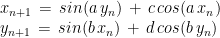
There are infinite attractors, since a, b, c and d are parameters. Given four values (one for each parameter) and a starting point (x0, y0), the previous equation defines the exact location of the point at step n, which is defined just by its location at n-1; an attractor can be thought as the trajectory described by a particle. This plot shows the evolution of a particle starting at (x0, y0)=(0, 0) with parameters a=-1.24458046630025, b=-1.25191834103316, c=-1.81590817030519 and d=-1.90866735205054 along 10 million of steps:

Changing parameters is really entertaining. Drawings have a sandy appearance:

From a technical point of view, the challenge is creating a data frame with all locations, since it must have 10 milion rows and must be populated sequentially. A very fast way to do it is using Rcpp package. To render the plot I use ggplot, which works quite well. Here you have the code to play with Clifford Attractors if you want:

library(Rcpp)
library(ggplot2)
library(dplyr)

opt = theme(legend.position  = "none",
            panel.background = element_rect(fill="white"),
            axis.ticks       = element_blank(),
            panel.grid       = element_blank(),
            axis.title       = element_blank(),
            axis.text        = element_blank())

cppFunction('DataFrame createTrajectory(int n, double x0, double y0, 
            double a, double b, double c, double d) {
            // create the columns
            NumericVector x(n);
            NumericVector y(n);
            x[0]=x0;
            y[0]=y0;
            for(int i = 1; i < n; ++i) {
            x[i] = sin(a*y[i-1])+c*cos(a*x[i-1]);
            y[i] = sin(b*x[i-1])+d*cos(b*y[i-1]);
            }
            // return a new data frame
            return DataFrame::create(_["x"]= x, _["y"]= y);
            }
            ')

a=-1.24458046630025
b=-1.25191834103316 
c=-1.81590817030519 
d=-1.90866735205054

df=createTrajectory(10000000, 0, 0, a, b, c, d)

png("Clifford.png", units="px", width=1600, height=1600, res=300)
ggplot(df, aes(x, y)) + geom_point(color="black", shape=46, alpha=.01) + opt
dev.off()

Chaotic Galaxies

Tell me, which side of the earth does this nose come from? Ha! (ALF)

Reading about strange attractors I came across with this book, where I discovered a way to generate two dimensional chaotic maps. The generic equation is pretty simple:

x_{n+1}= a_{1}+a_{2}x_{n}+a_{3}x_{n}^{2}+a_{4}x_{n}y_{n}+a_{5}y_{n}+a_{6}y_{n}^{2}
y_{n+1}= a_{7}+a_{8}x_{n}+a_{9}x_{n}^{2}+a_{10}x_{n}y_{n}+a_{11}y_{n}+a_{12}y_{n}^{2}

I used it to generate these chaotic galaxies:

Changing the vector of parameters you can obtain other galaxies. Do you want to try?

library(ggplot2)
library(dplyr)
#Generic function
attractor = function(x, y, z)
{
  c(z[1]+z[2]*x+z[3]*x^2+ z[4]*x*y+ z[5]*y+ z[6]*y^2, 
    z[7]+z[8]*x+z[9]*x^2+z[10]*x*y+z[11]*y+z[12]*y^2)
}
#Function to iterate the generic function over the initial point c(0,0)
galaxy= function(iter, z)
{
  df=data.frame(x=0,y=0)
  for (i in 2:iter) df[i,]=attractor(df[i-1, 1], df[i-1, 2], z)
  df %>% rbind(data.frame(x=runif(iter/10, min(df$x), max(df$x)), 
                          y=runif(iter/10, min(df$y), max(df$y))))-> df
  return(df)
}
opt=theme(legend.position="none",
          panel.background = element_rect(fill="#00000c"),
          plot.background = element_rect(fill="#00000c"),
          panel.grid=element_blank(),
          axis.ticks=element_blank(),
          axis.title=element_blank(),
          axis.text=element_blank(),
          plot.margin=unit(c(-0.1,-0.1,-0.1,-0.1), "cm"))
#First galaxy
z1=c(1.0, -0.1, -0.2,  1.0,  0.3,  0.6,  0.0,  0.2, -0.6, -0.4, -0.6,  0.6)
galaxy1=galaxy(iter=2400, z=z1) %>% ggplot(aes(x,y))+
  geom_point(shape= 8, size=jitter(12, factor=4), color="#ffff99", alpha=jitter(.05, factor=2))+
  geom_point(shape=16, size= jitter(4, factor=2), color="#ffff99", alpha=jitter(.05, factor=2))+
  geom_point(shape=46, size= 0, color="#ffff00")+opt
#Second galaxy
z2=c(-1.1, -1.0,  0.4, -1.2, -0.7,  0.0, -0.7,  0.9,  0.3,  1.1, -0.2,  0.4)
galaxy2=galaxy(iter=2400, z=z2) %>% ggplot(aes(x,y))+
  geom_point(shape= 8, size=jitter(12, factor=4), color="#ffff99", alpha=jitter(.05, factor=2))+
  geom_point(shape=16, size= jitter(4, factor=2), color="#ffff99", alpha=jitter(.05, factor=2))+
  geom_point(shape=46, size= 0, color="#ffff00")+opt
#Third galaxy
z3=c(-0.3,  0.7,  0.7,  0.6,  0.0, -1.1,  0.2, -0.6, -0.1, -0.1,  0.4, -0.7)
galaxy3=galaxy(iter=2400, z=z3) %>% ggplot(aes(x,y))+
  geom_point(shape= 8, size=jitter(12, factor=4), color="#ffff99", alpha=jitter(.05, factor=2))+
  geom_point(shape=16, size= jitter(4, factor=2), color="#ffff99", alpha=jitter(.05, factor=2))+
  geom_point(shape=46, size= 0, color="#ffff00")+opt
#Fourth galaxy
z4=c(-1.2, -0.6, -0.5,  0.1, -0.7,  0.2, -0.9,  0.9,  0.1, -0.3, -0.9,  0.3)
galaxy4=galaxy(iter=2400, z=z4) %>% ggplot(aes(x,y))+
  geom_point(shape= 8, size=jitter(12, factor=4), color="#ffff99", alpha=jitter(.05, factor=2))+
  geom_point(shape=16, size= jitter(4, factor=2), color="#ffff99", alpha=jitter(.05, factor=2))+
  geom_point(shape=46, size= 0, color="#ffff00")+opt

The Ikeda’s Galaxy

Chaos is the score upon which reality is written (Henry Miller)

Nonlinear dynamical systems are an enormous seam of amazing images. The Ikeda Map is an example of strange attractor which represents the movement of particles under the rules of certain differential equations.

I have drawn the trajectories followed by of 200 particles under the 2D-Ikeda Map with the same tecnique I used in this previous post, resulting this nice galaxy:

ikeda0.918

Wold you like to create your own galaxies? Here you have the code:

u=0.918 #Parameter between 0 and 1
n=200 #Number of particles
m=40 #Number of iterations
ikeda=data.frame(it=1,x1=runif(n, min = -40, max = 40), y1=runif(n, min = -40, max = 40))
ikeda$x2=1+u*(ikeda$x1*cos(0.4-6/(1+ikeda$x1^2+ikeda$y1^2))-ikeda$y1*sin(0.4-6/(1+ikeda$x1^2+ikeda$y1^2)))
ikeda$y2=  u*(ikeda$x1*sin(0.4-6/(1+ikeda$x1^2+ikeda$y1^2))+ikeda$y1*cos(0.4-6/(1+ikeda$x1^2+ikeda$y1^2)))
for (k in 1:m)
{
df=as.data.frame(cbind(rep(k+1,n),
ikeda[ikeda$it==k,]$x2,
ikeda[ikeda$it==k,]$y2,
1+u*(ikeda[ikeda$it==k,]$x2*cos(0.4-6/(1+ikeda[ikeda$it==k,]$x2^2+ikeda[ikeda$it==k,]$y2^2))-ikeda[ikeda$it==k,]$y2*sin(0.4-6/(1+ikeda[ikeda$it==k,]$x2^2+ikeda[ikeda$it==k,]$y2^2))),
u*(ikeda[ikeda$it==k,]$x2*sin(0.4-6/(1+ikeda[ikeda$it==k,]$x2^2+ikeda[ikeda$it==k,]$y2^2))+ikeda[ikeda$it==k,]$y2*cos(0.4-6/(1+ikeda[ikeda$it==k,]$x2^2+ikeda[ikeda$it==k,]$y2^2)))))
names(df)=names(ikeda)
ikeda=rbind(df, ikeda)
}
plot.new()
par(mai = rep(0, 4), bg = "gray12")
plot(c(0,0),type="n", xlim=c(-35, 35), ylim=c(-35,35))
apply(ikeda, 1, function(x) lines(x=c(x[2],x[4]), y=c(x[3],x[5]), col = paste("gray", as.character(min(round(jitter(x[1]*80/(m-1)+(20*m-100)/(m-1), amount=5)), 100)), sep = ""), lwd=0.1))