Now I’m gonna tell my momma that I’m a traveller, I’m gonna follow the sun (The Sun, Parov Stelar)
Inspired by this book I read recently, I decided to do this experiment. The idea is comparing how easy is to find sequences of numbers inside Pi, e, Golden Ratio (Phi) and a randomly generated number. For example, since Pi is 3.1415926535897932384… the 4-size sequence 5358 can be easily found at the begining as well as the 5-size sequence 79323. I considered interesting comparing Pi with a random generated number. What I though before doing the experiment is that it would be easier finding sequences inside the andom one. Why? Because despite of being irrational and transcendental I thought there should be some kind of residual pattern in Pi that should make more difficult to find random sequences inside it than do it inside a randomly generated number.
- I downloaded Pi, e and Phi from the Internet and extract first 100.000 digits of all of them. I generate a random 100.000 number on the fly.
- I generate a representative sample of 4-size sequences
- I look for each of these sequences inside first 5.000 digits of Pi, e, Phi and the randomly generated one. I repeat searching for first 10.000, first 15.000 and so on until I search into the whole 100.000 -size number
- I store how many sequences I find for each searching
- I repeat this for 5 and 6-size sequences.
At first sight, is equally easy (or difficult), to find random sequences inside all numbers: my hypothesis was wrong.
As you can see here, 100.000 digits is more than enough to find 4-size sequences. In fact, from 45.000 digits I reach 100% of successful matches:

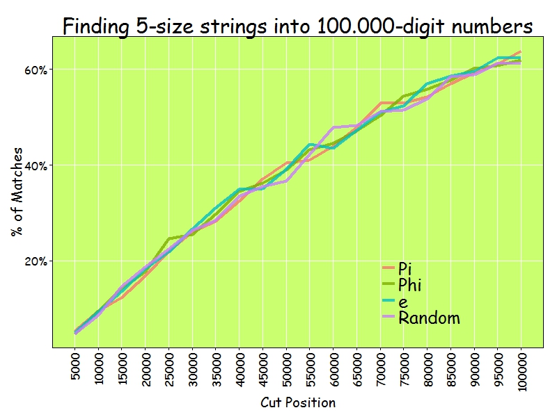
I only find 60% of 5-size sequences inside 100.000 digits of numbers:

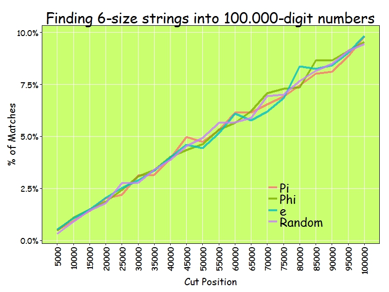
And only 10% of 6-size sequences:

Why these four numbers are so equal in order to find random sequences inside them? I don’t know. What I know is that if you want to find your telephone number inside Pi, you will probably need an enormous number of digits.
library(rvest)
library(stringr)
library(reshape2)
library(ggplot2)
library(extrafont);windowsFonts(Comic=windowsFont("Comic Sans MS"))
library(dplyr)
library(magrittr)
library(scales)
p = html("http://www.geom.uiuc.edu/~huberty/math5337/groupe/digits.html")
f = html("http://www.goldennumber.net/wp-content/uploads/2012/06/Phi-To-100000-Places.txt")
e = html("http://apod.nasa.gov/htmltest/gifcity/e.2mil")
p %>%
  html_text() %>%
  substr(., regexpr("3.14",.), regexpr("Go to Historical",.)) %>%
  gsub("[^0-9]", "", .)  %>%
  substr(., 1, 100000) -> p
f %>%
  html_text() %>%
  substr(., regexpr("1.61",.), nchar(.)) %>%
  gsub("[^0-9]", "", .) %>%
  substr(., 1, 100000) -> f
e %>%
  html_text() %>%
  substr(., regexpr("2.71",.), nchar(.)) %>%
  gsub("[^0-9]", "", .) %>%
  substr(., 1, 100000) -> e
r = paste0(sample(0:9, 100000, replace = TRUE), collapse = "")
results=data.frame(Cut=numeric(0), Pi=numeric(0), Phi=numeric(0), e=numeric(0), Random=numeric(0))
bins=20
dgts=6
samp=min(10^dgts*2/100, 10000)
for (i in 1:bins) {
  cut=100000/bins*i
  p0=substr(p, start=0, stop=cut)
  f0=substr(f, start=0, stop=cut)
  e0=substr(e, start=0, stop=cut)
  r0=substr(r, start=0, stop=cut)
  sample(0:(10^dgts-1), samp, replace = FALSE) %>% str_pad(dgts, pad = "0") -> comb
  comb %>% sapply(function(x) grepl(x, p0)) %>% sum() -> p1
  comb %>% sapply(function(x) grepl(x, f0)) %>% sum() -> f1
  comb %>% sapply(function(x) grepl(x, e0)) %>% sum() -> e1
  comb %>% sapply(function(x) grepl(x, r0)) %>% sum() -> r1
  results=rbind(results, data.frame(Cut=cut, Pi=p1, Phi=f1, e=e1, Random=r1))
}
results=melt(results, id.vars=c("Cut") , variable.name="number", value.name="matches")
opts=theme(
  panel.background = element_rect(fill="darkolivegreen1"),
  panel.border = element_rect(colour="black", fill=NA),
  axis.line = element_line(size = 0.5, colour = "black"),
  axis.ticks = element_line(colour="black"),
  panel.grid.major = element_line(colour="white", linetype = 1),
  panel.grid.minor = element_blank(),
  axis.text.y = element_text(colour="black"),
  axis.text.x = element_text(colour="black"),
  text = element_text(size=20, family="Comic"),
  legend.text = element_text(size=25),
  legend.key = element_blank(),
  legend.position = c(.75,.2),
  legend.background = element_blank(),
  plot.title = element_text(size = 30))
ggplot(results, aes(x = Cut, y = matches/samp, color = number))+
  geom_line(size=1.5, alpha=.8)+
  scale_color_discrete(name = "")+
  scale_x_continuous(breaks=seq(100000/bins, 100000, by=100000/bins))+
  scale_y_continuous(labels = percent)+
  theme(axis.text.x = element_text(angle = 90, vjust=.5, hjust = 1))+
  labs(title=paste0("Finding ",dgts, "-size strings into 100.000-digit numbers"),
       x="Cut Position",
       y="% of Matches")+opts