Category Archives: Curiosities

Mixing Benford, GoogleVis And On-Line Encyclopedia of Integer Sequences

The chess-board is the world; the pieces are the phenomena of the universe; the rules of the game are what we call the laws of Nature (T. H. Huxley)

One of the greatest packages I discovered recently is googleVis. While plotting with ggplot can be sometimes very arduous, doing plots with googleVis is extremely easy. Here you can find many examples of what you can do with this great package.

Not long ago, I also discovered The On-Line Encyclopedia of Integer Sequences (OEIS), a huge database of about 250.000 integer sequences where, for example, you can find the number of ways to lace a shoe that has n pairs of eyelets or the smallest number of stones in Tchoukaillon (or Mancala, or Kalahari) solitaire which make use of n-th hole. Many mathematicians, as Ralph Stephan, use this useful resource to develop their theories.

The third protagonist of this story is Frank Benford, who formulated in 1938 his famous law which states that considering different lists of numbers, 1 occurs as the leading digit about the 30% of time, while larger digits occur in that position less frequently.

In this experiment I read 20 random sequences from the OEIS. For each sequence, I obtain the distribution of first digit of the numbers and calculate the similarity with the theoretical distribution given by Benford’s Law so the more similar is the distribution, the closer is this number to 1. Sequences of OEIS are labeled with a seven characters code (an “A” followed by 6 digits). A nice way to show the output of this experiment is using the Gauge visualization of googleVis:

IMG1

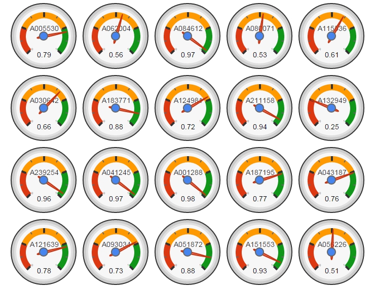
Sequence A001288 is the closest to the Benford’s Law. This sequence is the number of distinct 11-element subsets that can be formed from a n element set. Why is so close to the Benford’s Law? No idea further than binomial coefficients are related to some biological laws as number of descendants of a couple of rabbits.

I would like to wish you all a Merry Christmas and a Happy New Year:

library(plyr)
bendford=data.frame(first=0:9, freq=c(0,log10(1+1/(1:9))))
SequencesIds=formatC(sample(1:250000, 20, replace=FALSE), width = 6, format = "d", flag = "0")
results=data.frame(SEQID=character(0), BENDFORNESS=numeric(0))
for(i in 1:length(SequencesIds))
{
  SEQID = SequencesIds[i]
  TEXTFILE=paste("b", SEQID, ".txt", sep="")
  if (!file.exists(TEXTFILE)) download.file(paste("http://oeis.org/A",SEQID, "/b", SEQID, ".txt",sep=""), destfile = TEXTFILE)
  SEQ=readLines(paste("b", SEQID, ".txt", sep=""))
  SEQ=SEQ[SEQ != ""]
  SEQ=SEQ[unlist(gregexpr(pattern ='synthesized',SEQ))<0]
  m=t(sapply(SEQ, function(x) unlist(strsplit(x, " "))))
  df=data.frame(first=substr(gsub("[^0-9]","",m[,2]), 1, 1), row.names = NULL)
  df=count(df, vars = "first")
  df$freq=df$freq/sum(df$freq)
  df2=merge(x = bendford, y = df, by = "first", all.x=TRUE)
  df2[is.na(df2)]=0
  results=rbind(results, data.frame(SEQID=paste("A", SEQID, sep=""), BENDFORNESS=1-sqrt(sum((df2$freq.x - df2$freq.y) ^ 2))))
}
results$BENDFORNESS=as.numeric(format(round(results$BENDFORNESS, 2), nsmall = 2))
Gauge=gvisGauge(results, options=list(min=0, max=1, greenFrom=.75, greenTo=1, yellowFrom=.25, yellowTo=.75, redFrom=0, redTo=.25, width=400, height=300))
plot(Gauge)

The Awesome Parrondo’s Paradox

A technique succeeds in mathematical physics, not by a clever trick, or a happy accident, but because it expresses some aspect of physical truth (O. G. Sutton)

Imagine three unbalanced coins:

  • Coin 1: Probability of head=0.495 and probability of tail=0.505
  • Coin 2: Probability of head=0.745 and probability of tail=0.255
  • Coin 3: Probability of head=0.095 and probability of tail=0.905

Now let’s define two games using these coins:

  • Game A: You toss coin 1 and if it comes up head you receive 1€ but if not, you lose 1€
  • Game B: If your present capital is a multiple of 3, you toss coin 2. If not, you toss coin 3. In both cases, you receive 1€ if coin comes up head and lose 1€ if not.

Played separately, both games are quite unfavorable. Now let’s define Game A+B in which you toss a balanced coin and if it comes up head, you play Game A and play Game B otherwise. In other words, in Game A+B you decide between playing Game A or Game B randomly.

Starting with 0€, it is easy to simulate the three games along 500 plays. This is an example of one of these simulations:#Rstats #R

Resulting profit of Game A+B after 500 plays  is +52€ and is -9€ and -3€ for Games A and B respectively. Let’s do some more simulations (I removed legends and titles but colors of games are the same):

#Rstats #R

As you can see, Game A+B is the most profitable in almost all the previous simulations. Coincidence? Not at all. This is a consequence of the stunning Parrondo’s Paradox which states that two losing games can combine into a winning one.

If you still don’t believe in this brain-crashing paradox, following you can see the empirical distributions of final profits of three games after 1.000 plays:#Rstats #R

After 1000 plays, mean profit of Game A is -13€, is -7€ for Game B and 17€ for Game A+B.

This paradox was discovered in the last nineties by the Spanish physicist Juan Parrondo and can help to explain, among other things, why investing in losing shares can result in obtaining big profits. Amazing:

require(ggplot2)
require(scales)
library(gridExtra)
opts=theme(
  legend.position = "bottom",
  legend.background = element_rect(colour = "black"),
  panel.background = element_rect(fill="gray98"),
  panel.border = element_rect(colour="black", fill=NA),
  axis.line = element_line(size = 0.5, colour = "black"),
  axis.ticks = element_line(colour="black"),
  panel.grid.major = element_line(colour="gray75", linetype = 2),
  panel.grid.minor = element_blank(),
  axis.text.y = element_text(colour="gray25", size=15),
  axis.text.x = element_text(colour="gray25", size=15),
  text = element_text(size=20),
  plot.title = element_text(size = 35))
PlayGameA = function(profit, x, c) {if (runif(1) < c-x) profit+1 else profit-1}
PlayGameB = function(profit, x1, c1, x2, c2) {if (profit%%3>0) PlayGameA(profit, x=x1, c=c1) else PlayGameA(profit, x=x2, c=c2)}
####################################################################
#EVOLUTION
####################################################################
noplays=500
alpha=0.005
profit0=0
results=data.frame(Play=0, ProfitA=profit0, ProfitB=profit0, ProfitAB=profit0)
for (i in 1:noplays) {results=rbind(results, c(i,
    PlayGameA(profit=results[results$Play==(i-1),2], x =alpha, c =0.5),
    PlayGameB(profit=results[results$Play==(i-1),3], x1=alpha, c1=0.75, x2=alpha, c2=0.1),
    if (runif(1)<0.5) PlayGameA(profit=results[results$Play==(i-1),4], x =alpha, c =0.5) else PlayGameB(profit=results[results$Play==(i-1),4], x1=alpha, c1=0.75, x2=alpha, c2=0.1)
    ))}
results=rbind(data.frame(Play=results$Play, Game="A",   Profit=results$ProfitA),
              data.frame(Play=results$Play, Game="B",   Profit=results$ProfitB),
              data.frame(Play=results$Play, Game="A+B", Profit=results$ProfitAB))
ggplot(results, aes(Profit, x=Play, y=Profit, color = Game)) +
  scale_x_continuous(limits=c(0,noplays), "Plays")+
  scale_y_continuous(limits=c(-75,75), expand = c(0, 0), "Profit")+
  labs(title="Evolution of profit games along 500 plays")+
  geom_line(size=3)+opts
####################################################################
#DISTRIBUTION
####################################################################
noplays=1000
alpha=0.005
profit0=0
results2=data.frame(Play=numeric(0), ProfitA=numeric(0), ProfitB=numeric(0), ProfitAB=numeric(0))
for (j in 1:100) {results=data.frame(Play=0, ProfitA=profit0, ProfitB=profit0, ProfitAB=profit0)
  for (i in 1:noplays) {results=rbind(results, c(i,
      PlayGameA(profit=results[results$Play==(i-1),2], x =alpha, c =0.5),
      PlayGameB(profit=results[results$Play==(i-1),3], x1=alpha, c1=0.75, x2=alpha, c2=0.1),
      if (runif(1)<0.5) PlayGameA(profit=results[results$Play==(i-1),4], x =alpha, c =0.5)
      else PlayGameB(profit=results[results$Play==(i-1),4], x1=alpha, c1=0.75, x2=alpha, c2=0.1)))}
      results2=rbind(results2, results[results$Play==noplays, ])}
results2=rbind(data.frame(Game="A", Profit=results2$ProfitA),
data.frame(Game="B", Profit=results2$ProfitB),
data.frame(Game="A+B", Profit=results2$ProfitAB))
ggplot(results2, aes(Profit, fill = Game)) +
  scale_x_continuous(limits=c(-150,150), "Profit")+
  scale_y_continuous(limits=c(0,0.02), expand = c(0, 0), "Density", labels = percent)+
  labs(title=paste("Parrondo's Paradox (",as.character(noplays)," plays)",sep=""))+
  geom_density(alpha=.75)+opts

Hi

Why do some mathematicians wear a white coat? Are they afraid to be splashed by an integral? (Read on Twitter)

If you run into someone wearing a white coat who tells you something like

e raised to minus 3 by zero point five plus x squared plus y squared between two plus e raised to minus x squared minus y squared between two by cosine of four by x

do not be afraid: is just a harmless mathematician waving to you. Look at this:

HI2

This is the code to draw these mathematical greetings:

levelpersp=function(x, y, z, colors=heat.colors, ...) {
  ## getting the value of the midpoint
  zz=(z[-1,-1] + z[-1,-ncol(z)] + z[-nrow(z),-1] + z[-nrow(z),-ncol(z)])/4
  ## calculating the breaks
  breaks=hist(zz, plot=FALSE)$breaks
  ## cutting up zz
  cols=colors(length(breaks)-1)
  zzz=cut(zz, breaks=breaks, labels=cols)
  ## plotting
  persp(x, y, z, col=as.character(zzz), ...)
}
x=seq(-5, 5, length= 30);y=x
f=function(x,y) {exp(-3*((0.5+x)^2+y^2/2))+exp(-x^2-y^2/2)*cos(4*x)}
z=outer(x, y, f)
z[z>.001]=.001;z[z<0]=z[1,1]
levelpersp(x, y, z, theta = 30, phi = 55, expand = 0.5, axes=FALSE, box=FALSE, shade=.25)

Size Doesn’t Matter

An invisible red thread connects those destined to meet, regardless of time, place or circumstances. The thread may stretch or tangle, but never break (Ancient Chinese Legend)

I use to play once a year with my friends to Secret Santa (in Spain we call it Amigo Invisible). As you can read in Wikipedia:

Secret Santa is a Western Christmas tradition in which members of a group or community are randomly assigned a person to whom they anonymously give a gift. Often practiced in workplaces or amongst large families, participation in it is usually voluntary. It offers a way for many people to give and receive a gift at low cost, since the alternative gift tradition is for each person to buy gifts for every other person. In this way, the Secret Santa tradition also encourages gift exchange groups whose members are not close enough to participate in the alternative tradition of giving presents to everyone else.

To decide who gives whom, every year is the same: one of us introduces small papers in a bag with the names of participants (one name per paper). Then, each of us picks one paper and sees the name privately. If no one picks their own name,  the distribution is valid. If not, we have to start over. Every year we have to repeat process several times until obtaining a valid distribution. Why? Because we are victims of The Matching Problem.

Following the spirit of this talk I have done 16 simulations of the matching problem (for 10, 20, 30 … to 160 items). For example, given n items, I generate 5.000 random vectors sampling without replacement the set of natural numbers from 1 to n. Comparing these random vectors with the ordered one (1,2, …, n) I obtain number of matchings (that is, number of times where ith element of the random vector is equal to i). This is the result of the experiment:

matching

In spite of each of one represents a different number of matchings, all plots are extremely similar. All of them say that probability of not matching any two identical items is around 36% (look at the first bar of all of them). In concrete terms, this probability tends to 1/e (=36,8%) as n increases but does it very quickly.

This result is shocking. It means that if some day the 7 billion people of the world agree to play Secret Santa all together (how nice it would be!), the probability that at least one person chooses his/her own name is around 2/3. Absolutely amazing.

This is the code (note: all lines except two are for plotting):

library(ggplot2)
library(scales)
library(RColorBrewer)
library(gridExtra)
library(extrafont)
results=data.frame(size=numeric(0), x=numeric(0))
for (i in seq(10, by=10, length.out = 16)){results=rbind(results, data.frame(size=i, x=replicate(5000, {sum(seq(1:i)-sample(seq(1:i), size=i, replace=FALSE)==0)})))}
opts=theme(
  panel.background = element_rect(fill="gray98"),
  panel.border = element_rect(colour="black", fill=NA),
  axis.line = element_line(size = 0.5, colour = "black"),
  axis.ticks = element_line(colour="black"),
  panel.grid.major.y = element_line(colour="gray80"),
  panel.grid.major.x = element_blank(),
  panel.grid.minor = element_blank(),
  axis.text.y = element_text(colour="gray25", size=15),
  axis.text.x = element_text(colour="gray25", size=15),
  text = element_text(family="Humor Sans", size=15, colour="gray25"),
  legend.key = element_blank(),
  legend.position = "none",
  legend.background = element_blank(),
  plot.title = element_text(size = 18))
sizes=unique(results$size)
for (i in 1:length(sizes))
{
  data=subset(results, size==sizes[i])
  assign(paste("g", i, sep=""),
         ggplot(data, aes(x=as.factor(x), weight=1/nrow(data)))+
           geom_bar(binwidth=.5, fill=sample(brewer.pal(9,"Set1"), 1), alpha=.85, colour="gray50")+
           scale_y_continuous(limits=c(0,.4), expand = c(0, 0), "Probability", labels = percent)+
           scale_x_discrete(limit =as.factor(0:8), expand = c(0, 0), "Number of matches")+
           labs(title = paste("Matching", as.character(sizes[i]), "items ...", sep=" "))+
           opts)
}
grid.arrange(g1, g2, g3, g4, g5, g6, g7, g8, g9, g10, g11, g12, g13, g14, g15, g16, ncol=4)

Princess Jasmine’s Trick

I’m history! No, I’m mythology! Nah, I don’t care what I am; I’m free hee! (Genie, when he is released from the magical oil lamp by Aladdin)

Princess JasmineA long time ago, in a kingdom far away, lived a beautiful princess named Jasmine. There also lived a very rich and evil wizard named Jafar, who was in love with the princess. In order to married with Jasmine, Jafar bought  her father’s will with treasures, but the princess was harder to convince. One day Jafar told the princess: Request me whatever you want and if  I am able to bring it to you, you will become my wife. The princess, tired of the insistence of Jafar, answered: I only want a gold chain, but I want you to give it to me as follows: the first day I should have just one link of the chain. The second day I should have two links. The third day, three … and so on. When you give me all the links of the chain I will marry you. Jafar, intrigued, asked: But how many links should have the chain?  And Jasmine replied: I want you to give me the longest chain that allows you to pay me breaking only 30 links. Jafar began to laugh out loud as he walked away and said to the princess: Tomorrow I’ll bring you such chain!. But as he went to his palace, his happiness turned into anger: he realized that there was not enough gold in the world to build the chain that asked Jasmine.

This is my own version of one of my favorite anti-common-sense mathematical curiosities. To explain it, let me start with an example. Imagine a simple chain with 7 links. If you open the 3rd link, the you split the chain into 3 pieces: a single link (the one you opened), a piece of 2 links and another one of 4 links. You could pay to Jasmine during seven days combining these 3 pieces:

  • Day 1: Give her the single link
  • Day 2: Give her the 2-links piece and take the single link, leaving her with 2 links
  • Day 3: Give her the single link again, leaving her with 3 links
  • Day 4: Give her the 4-links piece and take all pieces she has, leaving her with 4 links
  • Day 5: Give her the single link again, leaving her with 5 links
  • Day 6: Give her the 2-links piece and take 2-links piece, leaving her with 6 links
  • Day 7: Give her the single link piece, leaving her with all links

Is easy to see that having a chain with 63 links, you could pay Jasmine breaking only 3 links (positions 5th, 14th and 31st). It easy to prove that the length of the biggest chain you can manage breaking only n links is (2n+1-1)*(n+1)+n

Next plot represents the minimum number of breaks to pay Jasmine daily for a given chain’s length. I call it the Jasmine’s Staircase:

Generated With R #rstats

Some curiosities around chains:

  • Jasmine asked Jafar a chain of 66.571.993.087 links
  • Supposing one link weights 4 grams, the chain of Jasmine would weight around 266 tons. It is supposed to be around 171 tons of gold in the world
  • If you spend 1 second to climb the first step of the staircase, you will spend 302 years to climb the step number 100

Jafar was right. Jasmine was clever:

library(sqldf)
library(ggplot2)
library(extrafont)
max.breaks=5
CalculateLength = function(n) {n+sum(sapply(0:n, function(x) 2^x*(n+1)))}
results=data.frame(breaks=1:max.breaks, length=sapply(1:max.breaks, CalculateLength))
links=data.frame(links=2:CalculateLength(max.breaks))
results=sqldf("SELECT links.links, min(results.breaks) as minbreaks FROM links, results WHERE links.links <= results.length GROUP BY 1")
opts=theme(
panel.background = element_rect(fill="mistyrose"),
panel.border = element_rect(colour="black", fill=NA),
axis.line = element_line(size = 0.5, colour = "black"),
axis.ticks = element_line(colour="black"),
panel.grid = element_line(colour="white", linetype = 2),
axis.text.y = element_text(colour="black"),
axis.text.x = element_text(colour="black"),
text = element_text(size=20, family="Humor Sans"),
plot.title = element_text(size = 40)
)
ggplot(results, aes(links,minbreaks))+
geom_area(fill="violet", alpha=.4)+
geom_step(color="violetred", lwd=1.5)+
labs(x="Chain's Length", y="Minimum Number of Breaks", title="Princess Jasmine's Staircase")+
scale_x_continuous(expand = c(0, 0), breaks = sapply(1:max.breaks, CalculateLength))+
opts

The Zebra Of Riemann

Mathematics is the art of giving the same name to different things (Henri Poincare)

Many surveys among experts point that demonstration of the Riemann Hypothesis is the most important pending mathematical issue in this world. This hypothesis is related to Riemann zeta function, which is supossed to be zero only for those complex whose real part is equal to 1/2 (this is the conjecture of Riemann itself). Confirming the conjecture would imply deep consequences in prime numbers teory and also in our knowledge of their properties. Next plot represents the argument of zeta function over complex with real part between -75 and 5 (x axis) and imaginary part between -40 and 40 (y axis). An explanation of this kind of graph can be found here. Does not it remind you of something?
zebra
Solving the hypothesis of Riemann is one of the seven Clay Mathematics Institute Millennium Prize Problems. Maybe zebras keep the secret to solve it in their skins.

This is the code to plot the graph:

require(pracma)
z=outer(seq(-75, 5, by =.1),1i*seq(-40, 40, by =.1),'+')
z=apply(z, c(1,2), function(x) Arg(zeta(x)))
opt=theme(legend.position="none",
panel.background = element_blank(),
panel.grid = element_blank(),
axis.ticks=element_blank(),
axis.title=element_blank(),
axis.text =element_blank())
z=data.frame(expand.grid(x=seq(ncol(z)), y=seq(nrow(z))), z=as.vector(z))
require(ggplot2)
ggplot(z, aes(x=x, y=y, color=z)) + geom_tile() + scale_colour_gradientn(colours=c("black","white", "gray80", "gray40")) + opt

How To Approximate Pi With A Short Pencil And A Big Paper

Experiment, be curious: though interfering friends may frown, get furious at each attempt to hold you down (Tony Bennett, Experiment)

Instructions:

  1. Take a pencil and measure it
  2. Take a piece of paper and draw parallel lines on it (you can use the pencil, of course); separation between lines should double the length of the pencil
  3. Toss the pencil over the paper 100 times (or more)
  4. Make note of how many times do the pencil cross some of the lines
  5. Calculate ratio between tosses and crosses: this is your approximation of Pi

Some time ago, I published a post about one of the most amazing places where PI was discovered. This is another example of the ubiquity of this mathematical constant. This experiment is based on Buffon’s needle problem, another amazing experiment of 18th century. Next plot represents ratio of tosses to crosses depending on the length of pencil. When the pencil is half the length of the separation between lines, the previous ratio is approximately PI:
Buffon
If you get very bored some afternoon you can replicate this experiment with your children. Use a short pencil. If not, you will need an extremely big piece of paper. Meanwhile here you have the code:

trials=100000
results=sapply(seq(.1, 2, by = .05), function(x)
{
  r=x #Length of pencil in relation to separation between lines
  Needles=t(sapply(1:trials, function(y) c(100*runif(1),2*pi*runif(1))))
  Needles=cbind(Needles,Needles[,1]+r*cos(Needles[,2]))
  Needles=data.frame(x1=Needles[,1], x2=Needles[,3], Cross=abs(trunc(Needles[,1])-trunc(Needles[,3])))
  c(r, trials/(trials-nrow(Needles[Needles$Cross==0,])))
})
results=data.frame(t(results))
colnames(results)=c(c("ratio", "inv.perc.crosses"))
require(ggplot2)
require(extrafont)
require(grid)
opts=theme(
  panel.background = element_rect(fill="darkolivegreen1"),
  panel.border = element_rect(colour="black", fill=NA),
  axis.line = element_line(size = 0.5, colour = "black"),
  axis.ticks = element_line(colour="black"),
  panel.grid.major = element_line(colour="white", linetype = 1),
  panel.grid.minor = element_blank(),
  axis.text.y = element_text(colour="black", size=20),
  axis.text.x = element_text(colour="black", size=20),
  text = element_text(size=25, family="xkcd"),
  legend.key = element_blank(),
  legend.position = c(.2,.75),
  legend.background = element_blank(),
  plot.title = element_text(size = 50))
c=ggplot(results, aes(ratio, inv.perc.crosses))
c +geom_abline(intercept = pi, slope = 0, size = 0.4, linetype=2, colour = "black", alpha=0.8)+
  geom_line(color="green4", size=1.5)+
  geom_point(color="gray92", size=8, pch=16)+
  geom_point(color="green4", size=6, pch=16)+
  geom_text(aes(0.55, 5), hjust=0, family="xkcd", label="PI is around here!", size=10)+
  ggtitle("Hot to approximate PI with \na short pencil and a big paper")+
  xlab("Length of pencil divided by separation between lines") +
  ylab("Number of tosses divided by number of crosses")+
  geom_segment(aes(x = .625, y = 4.6, xend = .52, yend = 3.45), size=1.5, arrow = arrow(length = unit(0.5, "cm")))+
  scale_y_continuous(breaks=c(pi, 4, 8, 12, 16), labels=c("3.141593","4","8","12","16"))+
  scale_x_continuous(breaks=seq(.1, 2, by = .1))+opts

The Gilbreath’s Conjecture

317 is a prime, not because we think so, or because our minds are shaped in one way rather than another, but because it is so, because mathematical reality is built that way (G.H. Hardy)

In 1958, the mathematician and magician Norman L. Gilbreath presented a disconcerting hypothesis conceived in the back of a napkin. Gilbreath wrote first prime numbers in a row. In the next rows, he wrote the difference  in absolute value of consecutive values of previous row. Beginning with first 20 primes in the first row, he obtained something like this:Gilbreath01

The conjecture is easy: except for the first one, all elements of the first column are 1. So far, no one has demonstrated this hypothesis. In fact, according to mathematician Richard Guy, it seems unlikely that we will see a demonstration of Gilbreath’s conjecture in the near future, though probably this conjecture is true.

In the previous chart, I coloured zeros in white, ones in violet and rest of numbers in gold. The conjecture says that except for the first element, the first column is entirely violet. Following you can see the coloured chart for first 20, 40, 60 and 80 prime numbers:

Gilbreath02

It is nice how zeros create triangular patterns similar to patterns created by cellular automata. This is the chart for first 200 primes:Gilbreath03

How much time will it take to demonstrate this simple conjecture? Who knows. Meanwhile, you can draw triangles with this code:

library(ggplot2)
create.gilbreath=function(n)
{
require(reshape)
require(schoolmath)
data(primlist)
gilbreath=t(matrix(primlist[2:(n+1)], n, n))
for (i in 2:n) {gilbreath[i,]=c(eval(parse(text=paste(c(paste("abs(diff(",collapse=""), "gilbreath[i-1,]", paste("))",collapse="")),collapse=""))),rep(NA,1))}
na.omit(melt(t(gilbreath)))
}
opt=theme(legend.position="none",
panel.background = element_blank(),
panel.grid = element_blank(),
axis.ticks=element_blank(),
axis.title=element_blank(),
axis.text =element_blank())
gilbreath=create.gilbreath(20)
gilbreath$value1=cut(gilbreath$value, breaks=c(-Inf,1:2,Inf), right = FALSE)
ggplot(gilbreath, aes(x=X1, y=X2)) +
geom_tile(aes(fill = value1), colour="grey") +
scale_fill_manual(values = c("white", "darkviolet", "gold"))+
geom_text(label=gilbreath$value, size=8)+
scale_y_reverse()+opt

The Three Little Pigs

Jesse, you asked me if I was in the meth business or the money business. Neither. I’m in the empire business (Walter White in Breaking Bad)

The game of pig has simple rules but complex strategies. It was described for the first time in 1945  by a magician called John Scarne. Playing the pig game is easy: each turn, a player repeatedly rolls a die until either a 1 is rolled or the player decides to hold:

  • If the player rolls a 1, they score nothing and it becomes the next player’s turn
  • If the player rolls any other number, it is added to their turn total and the player’s turn continues
  • If a player chooses to hold, their turn total is added to their score, and it becomes the next player’s turn

The first player who reach at least 100 points is the winner. For example: you obtain a 3 and then decide to roll again, obtaining a 1. Your score is zero in this turn. Next player gets the sequence 3-4-6 and decides to hold, obtaining a score of 13 points in this turn.

Despite its simplicity, the pig game has a very complex and against-intuition optimal strategy. It was calculated in 2004 by Todd W. Neller and Clifton Presser from Gettysburg College of Pennsilvania with the help of computers.

To illustrate the game, I simulated three players (pigs) playing the pig game with three different strategies:

  • The Coward pig, who only rolls the die a small number of times in every turn
  • The Risky pig, who rolls the die a more times than the coward one
  • The Ambitious pig, who tries to obtain in every turn more points than two others

I simulated several scenarios.

  • Some favorable scenarios for Coward pig:

pigs2Coward pigs4Coward

In first scenario, the Coward pig rolls the die between 1 and 5 times each round and wins if the Risky pig asumes an excessive level of risk (rolling each time between 10 and 15 times). Trying to obtain more than the Coward is a bad option for the Ambitious pig. Simulating this scenario 100 times gives victory to Coward a 51% of times (25% to Risky and 24% to Ambitious).

Second scenario puts closer Coward and Risky pigs (first one rolls the die between 4 and 7 times  each round and second one between 6 and 9 times). Coward wins 54% of times (34% Risky and only 12% Ambitious).

Being coward seems to be a good strategy when you play against a reckless or when you are just a bit more conservative than a Risky one.

  • Some favorable scenarios for Risky pig:

pigs5RiskyPigs1Risky

Rolling the die between 4 and 6 times each round seems to be a good option, even more when you are playing against a extremely conservative player who rolls no more than 3 times each time. Simulating 100 times these previous scenarios gives victory to Risky pig a 58% of times in first the case in which Coward rolls allways 1 and Risky 6 times each round (0% for Coward and only 42% form Ambitious) and 66% of times in the second one (only 5% to Coward and 29% to Ambitious).

Being Risky is a good strategy when you play against a chicken.

  • Some favorable scenarios for Ambitious pig:

pigs3Ambitious pigs6ambitious

The Ambitious pig wins when two others turn into extremely coward and risky pigs as can be seen in the first scenario in which Ambitious wins 65% of the times (31% for Coward and 4% for Risky). Ambitious pig also wins when two others get closer and hit the die a small number of times (2 rolls the Coward and 4 rolls the Risky). In this scenario the Ambitious wins 58% of times (5% for Coward and 37% for Risky). By the way, these two scenarios sound very unreal.

Being ambitious seems to be dangerous but works well when you play against a crazy and a chicken or against very conservative players.

From my point of view, this is a good example to experiment with simulations, game strategies and xkcd style graphics.

The code:

require(ggplot2)
require(extrafont)
#Number of hits for Coward
CowardLower=2
CowardUpper=2
#Number of hits for Risky
RiskyLower=4
RiskyUpper=4
game=data.frame(ROUND=0, part.p1=0, part.p2=0, part.p3=0, Coward=0, Risky=0, Ambitious=0)
while(max(game$Coward)<100 & max(game$Risky)<100 & max(game$Ambitious)<100)
{
#Coward Little Pig
p1=sample(1:6,sample(CowardLower:CowardUpper,1), replace=TRUE)
s1=min(min(p1-1),1)*sum(p1)
#Risky Little Pig
p2=sample(1:6,sample(RiskyLower:RiskyUpper,1), replace=TRUE)
s2=min(min(p2-1),1)*sum(p2)
#Ambitious Little Pig
s3=0
repeat {
p3=sample(1:6,1)
s3=(p3+s3)*min(min(p3-1),1)
if (p3==1|s3>max(s1,s2)) break
}
game[nrow(game)+1,]=c(max(game$ROUND)+1,s1,s2,s3,max(game$Coward)+s1,max(game$Risky)+s2,max(game$Ambitious)+s3)
}
opts=theme(
panel.background = element_rect(fill="darkolivegreen1"),
panel.border = element_rect(colour="black", fill=NA),
axis.line = element_line(size = 0.5, colour = "black"),
axis.ticks = element_line(colour="black"),
panel.grid.major = element_line(colour="white", linetype = 1),
panel.grid.minor = element_blank(),
axis.text.y = element_text(colour="black"),
axis.text.x = element_text(colour="black"),
text = element_text(size=25, family="xkcd"),
legend.key = element_blank(),
legend.position = c(.2,.75),
legend.background = element_blank(),
plot.title = element_text(size = 50)
)
ggplot(game, mapping=aes(x=game$ROUND, y=game$Coward)) +
geom_line(color="red", size=1.5) +
geom_line(aes(x=game$ROUND, y=game$Risky), color="blue", size=1.5) +
geom_line(aes(x=game$ROUND, y=game$Ambitious), color="green4", size=1.5) +
geom_point(aes(x=game$ROUND, y=game$Coward, colour="c1"), size=5.5) +
geom_point(aes(x=game$ROUND, y=game$Risky, colour="c2"), size=5.5) +
geom_point(aes(x=game$ROUND, y=game$Ambitious, colour="c3"), size=5.5) +
ggtitle("THE THREE LITTLE PIGS") +
xlab("ROUND") + ylab("SCORING") +
geom_text(aes(max(game$ROUND), max(max(game$Coward, game$Risky, game$Ambitious)), hjust=1.2, family="xkcd", label="WINNER!"), size=10)+
geom_hline(yintercept=100, linetype=2, size=1)+
scale_y_continuous(breaks=seq(0, max(max(game$Coward, game$Risky, game$Ambitious))+10, 10))+
scale_x_continuous(breaks=seq(0, max(game$ROUND), 1))+
scale_colour_manual("",
labels = c(paste("Coward: ", CowardLower, "-", CowardUpper, " hits", sep = ""), paste("Risky: ", RiskyLower, "-", RiskyUpper, " hits", sep = ""), "Ambitious"),
breaks = c("c1", "c2", "c3"),
values = c("red", "blue", "green4"))+ opts

floweR

It is the time you have wasted for your rose that makes your rose so important (Antoine de Saint-Exupéry, The Little Prince)

Yesterday I found a package called circular and I could not suppress to do this:

rose

Make your own floweRs:

require(circular)
for (i in 1:8)
{
  rose.diag(circular(runif(5000, 0, 2*pi)), 
            bins = (25-round(abs(jitter(0, amount=2*i)))), 
            axes=FALSE,
            border=rgb(255,50+204*((i-1)/8),50+204*((i-1)/8), alpha=255, max=255),
            ticks = FALSE,
            col=rgb(250,0+204*((i-1)/8),0+204*((i-1)/8), alpha=255, max=255), 
            control.circle=circle.control(lty=0), 
            shrink=0.22+(i-1)*(2-0.22)/8)
  par(new=TRUE)  
}
for (i in 1:150)
  {
  q = runif(1)*pi*2
  r = sqrt(runif(1))
  x = (0.18*r)* cos(q)
  y = (0.18*r)* sin(q)
  points(x, y, 
         col = rgb(255 ,sample(80:120, 1), 0, alpha= 95, max=255),
         bg = rgb(255 ,sample(100:200, 1), 0, alpha= 95, max=255), pch=21, cex=2)
  }