Category Archives: Cellular Automata

Neighborhoods: Experimenting with Cyclic Cellular Automata

On candy stripe legs the Spiderman comes, softly through the shadow of the evening sun (Lullaby, The Cure)

Cellular automata are an inmense source of artistical images. Today, I experimented with Cyclic automata, which are ruled with these simple rules:

  • Create a grid of cells.
  • Give a state to each cell randomly; states a numbers between 0 and M-1 (you choose the value of M previously).
  • For each cell, count how many of its neighbouring cells have their state value exactly 1 unit greater than the cell’s state.
  • If the resulting number is greater than a certain thresold (that you also choose previously) increment the state of the cell by 1; if cell state reaches value of M, then you have to put 0 (in other words, you have to add 1 modulus M).
  • Repeat two previous steps a number of times.

A key concept in this algorithm is defining which is the neighborhood of a cell. There are two of them quite famous: Moore and Von Neumann neighborhoods, but you can define your own ones. Once you decide to stop iterating, you can give color to each cell according its final state, and you will obtain images like this one:

If you have a look to the code, you will see the next parameters:

  • neighborhood: the pattern of neighbouring cells
  • range: the depth of neighborhood
  • states: maximum number of states allowed (the M of the algorithm)
  • thresold
  • iter: number of iterations
  • width and height of the grid

Apart from Moore and Von Neumann, I implemented some other neighborhoods. This chart shows some of them. In columns you can find the folowing: M (Moore), N (Von Neumann), Mr (Moore remote), Nr (Von Neumann remote), Cr (Cross), S1 (S-Shape #1), Bl (Blade), C2 (Corners #2) and TM (Tick Mark). In rows, you can find different ranges for each neighborhood, from 1 to 4:

You will find more neighborhood in the code of the experiment, which is here. There are infinite combinations of the previous parameters, and each one results in a different image:


I used again COLOULovers palettes As always, I encourage you to experiment with the code, create your own neighborhoods, and see how they work. Happy New Year 2021!

Abstractions

Spinning on that dizzy edge (Just Like Heaven, The Cure)

This post talks about a generative system called Physarum model, which simulates the evolution of a colony of extremely simple organisms that, under certain environmental conditions, result into complex behaviors. Apart from the scientific interest of the topic, this model produce impressive images like this one, that I call The Death of a Red Dwarf:

You can find a clear explanation of how a physarum model works in this post, by Sage Jenson. A much deeper explanation can be found in this paper by Jeff Jones, from the University of the West of England. Briefly, a physarum model evolves a set of particles (agents), making them move over a surface. Agents turn towards locations with higher concentrations of a pheromone trail. Once they move, they make a deposition of pheromone as well. These are the steps of a single iteration of the model:

  • Sensor stage: Each agent looks to three positions of the trail map (left, front and right) according a certain sensor angle
  • Motor stage: then it moves to the place with the higher concentration with some rules to deal with ties
  • Deposition stage: once in the new location, the agent deposites a certain amount of pheromone.
  • Diffuse stage: the pheromones diffusing over the surface to blur the trail array.
  • Decay stage: this make to decay the concentration of pheromone on the surface.

Sage Jenson explains the process with this illustrative diagram:

My implementation is a bit different from Jones’ one. The main difference is that I do not apply the diffuse stage after deposition: I prefer a high defined picture instead blurriyng it. I also play with the initial arrangement of agents (location and heading angle) as well with the initial configuration of environment. For example, In The Death of a Red Dwarf, agents start from a circle and the environment is initialized in a dense disc. You can find the details in the code. There you will see that the system is governed by the following parameters:

  • Front and left sensor angles from forward position
  • Agent rotation angle
  • Sensor offset distance
  • Step size (how far agent moves per step)
  • Chemoattractant deposition per step
  • Trail-map chemoattractant diffusion decay factor

In adition to them (specific of the physarum model), you also can change others like colors, noise of angles (parameter amount of jitter function), number of agents and iterations as well as the initial arrangement of the environment and the location of agents. I invite you to do it. You will discover many abstractions: butterfly wings, planets, nets, explosions, supernovas … I have spent may hours playing with it. Some examples:

You can find the code here. Please, let me know if you do something interesting with it. Share your artworks with me in Twitter or drop me an email (you can find my address here).

Watercolors

Moça do corpo dourado
Do Sol de Ipanema
O seu balançado
É mais que um poema
(Garota de Ipanema, João Gilberto)

Sometimes I think about the reasons why I spend so many time doing experiments and writing my discoveries in a blog. Even although the main reason to start this blog was some kind of vanity, today I have pretty clear why I still keep writing it: to keep my mind tuned. I really enjoy looking for ideas, learning new algorithms, figuring out the way to translate them into code and trying to discover new territories going a step further. I cannot imagine my life without coding. Many good times in the last years have been in front of my laptop listening music and drinking a beer. In these strange times, confined at house, coding has became in something more important. It keeps me ahead from the sad news and moves my mind to places where everything is quiet, friendly and perfect. Blogging is my therapy, my mindfulness.

This post is inspired in this post from Softology, an amazing blog I recommend you to read. In it, you can find a description of the stepping stone cellular automaton as well as a appealing collection of images generated using this technique. I modified the original algorithm described in the post to create images like these, which remind me a watercolor painting:

I begin with a 400 x 400 null matrix. After that, I choose a number of random pixels that will act as centers of circles. Around them I substitute the initial zeros by numbers drawned from a normal distribution which mean depends on the distance of pixels to the center. The next step is to apply the stepping stone algorithm. For each pixel, I substitute its value by a weighted average of itself and the value of some of its neighbors, choosen randomly. I always mix values of the pixels. The original algorithm, as described in the Softology’s blog, performs these mixings randomly. Another difference is that I mix values intead interchanging them, as the original algorithm does. Once I repeat this process a number of times, I pick a nice palette from COLOURLovers and turn values of pixels into colors with ggplot:

The code is here. Let me know if you do something interesting with it. Turning numbers into bright colors: I cannot imagine a better way to spend some hours in these shadowy times.

Looking For Life


Machines take me by surprise with great frequency (Alan Turing)

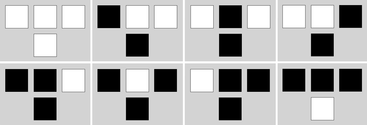
Imagine a 8×8 grid in which cells can be alive (black colored) or empty (light gray colored): Generated with R #RstatsAs with the One-dimensional Cellular Automata, the next state of a cell is a function of the states of the cell’s nearest neighbors (the only neighbors that we consider are the eight cells that form the immediate perimeter of a cell). To evolve this community of cells over time, rules are quite simple:

  • If a live cell has less than two neighbors, then it dies (loneliness)
  • If a live cell has more than three neighbors, then it dies (overcrowding)
  • If an dead cell has three live neighbors, then it comes to life (reproduction)
  • Otherwise, a cell stays as is (stasis)

These are the rules of the famous Conway’s Game Of Life, a cellular automaton invented in the late 1960s by John Conway trying to refine the description of a cellular automaton to the simplest one that could support universal computation. In 1970 Martin Gardner described Conway’s work in his Scientific American column. Gardner’s article inspired many people around the world to experiment with Conway’s, which eventually led to the final pieces of how the Game Of Life could support universal computation in what was surely a global collaborative effort.

In this experiment I will try to find interesting objects that can be found in the Game Of Life: static (remain the same over the time), periodic (change but repeating their initial configuration in some iterations) or moving objects (travel through the grid before disappearing). Why are interesting? Because these are the kind of objects required to perform computations.

The plan is simple: I will generate some random grids and will evolve them over time a significant number of times. After doing this, I will check those grids having still some alive cells inside. Will I find there what I am looking for?

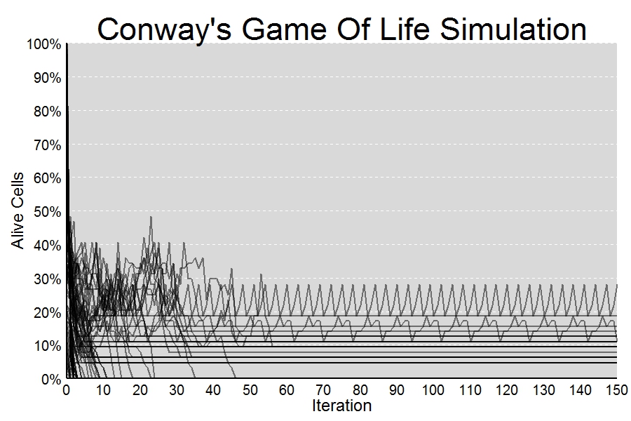
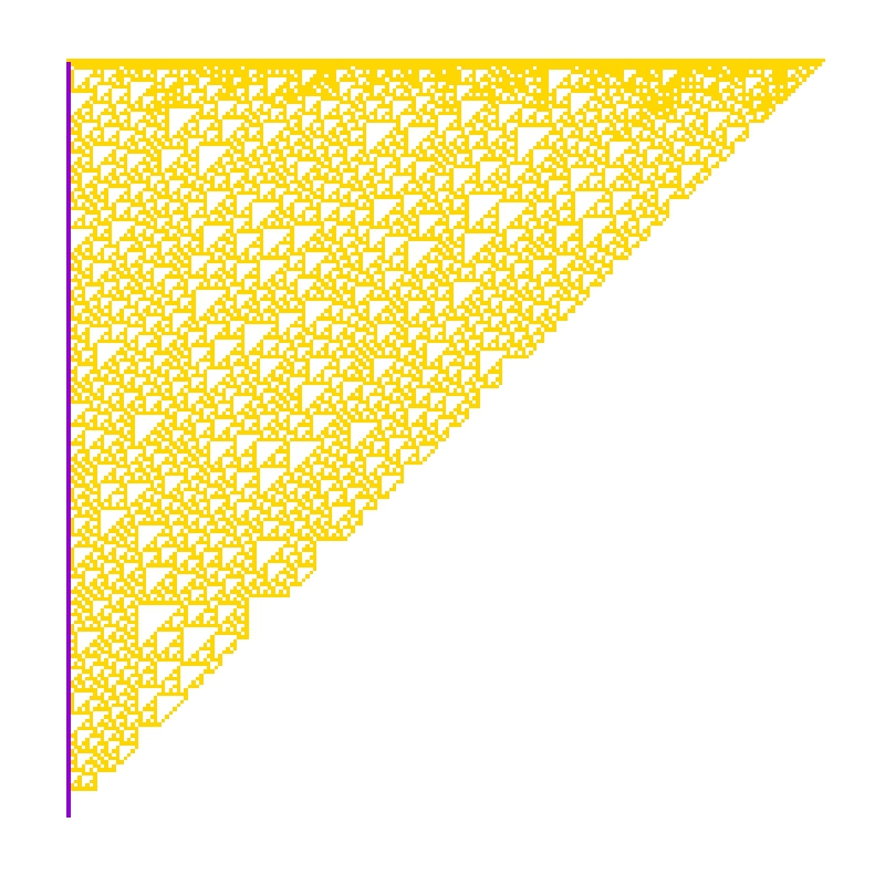
I generated 81 grids in which live cells are randomly located using binomial random variables with probabilities equal to i/80 with i from 0 (all cells empty) to 80 (all cells alive). This is a quick way to try a set of populations with a wide range of live cells. I measure % of alive cells after each iteration. I will analyze those grids which still have live cells after all iterations. This is what happens after 150 iterations:

Generated with R #Rstats

I find some interesting objects. Since I keep them in my script, I can list them with ls(pattern= "Conway", all.names = TRUE). Two of them are specially interesting because are not static. Are those which produce non-constant lines in the previous plot.

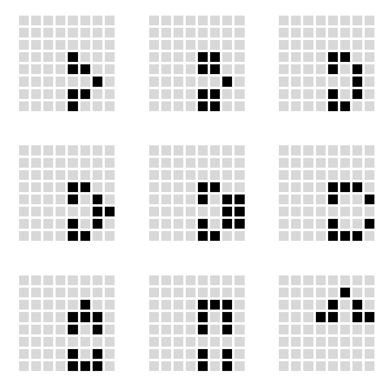
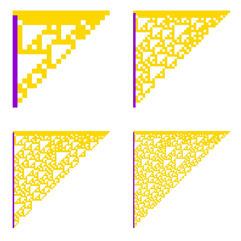
First one is a periodic object which reproduces itself after every 3 iterations:

Generated with R #Rstats

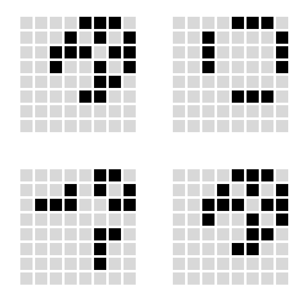
Second one is a bit more complex. After 8 iterations appears rotated:

Generated with R #Rstats

What kind of calculations can be done with these objects? I don’t now yet but let’s give time to time. Do you want to look for Life?

library(ggplot2)
library(scales)
library(gridExtra)
SumNeighbors = function (m) #Summarizes number of alive neighbors for each cell
{
  rbind(m[-1,],0)+rbind(0,m[-nrow(m),])+cbind(m[,-1],0)+cbind(0,m[,-ncol(m)])+
    cbind(rbind(m[-1,],0)[,-1],0)+cbind(0, rbind(0,m[-nrow(m),])[,-nrow(m)])+
    cbind(0,rbind(m[-1,],0)[,-nrow(m)])+cbind(rbind(0,m[-nrow(m),])[,-1],0)
}
NextNeighborhood = function (m) #Calculates next state for each cell according to Conway's rules
{
  (1-(SumNeighbors(m)<2 | SumNeighbors(m)>3)*1)-(SumNeighbors(m)==2 & m==0)*1
}
splits=80 #Number of different populations to simulate. Each population s initialized randomly
          #according a binomial with probability i/splits with i from 0 to splits
iter=150
results=data.frame()
rm(list = ls(pattern = "conway")) #Remove previous solutions (don't worry!)
for (i in 0:splits)
{
  z=matrix(rbinom(size=1, n=8^2, prob=i/splits), nrow=8); z0=z
  results=rbind(results, c(i/splits, 0, sum(z)/(nrow(z)*ncol(z))))
  for(j in 1:iter)
  {z=NextNeighborhood(z); results=rbind(results, c(i/splits, j, sum(z)/(nrow(z)*ncol(z))))}
  #Save interesting solutions
  if (sum(z)/(nrow(z)*ncol(z))>0) assign(paste("Conway",format(i/splits, nsmall = 4), sep=""), z)
}
colnames(results)=c("start", "iter", "sparsity")
#Plot reults of simulation
opt1=theme(panel.background = element_rect(fill="gray85"),
          panel.grid.minor = element_blank(),
          panel.grid.major.x = element_blank(),
          panel.grid.major.y = element_line(color="white", size=.5, linetype=2),
          plot.title = element_text(size = 45, color="black"),
          axis.title = element_text(size = 24, color="black"),
          axis.text = element_text(size=20, color="black"),
          axis.ticks = element_blank(),
          axis.line = element_line(colour = "black", size=1))
ggplot(results, aes(iter, sparsity, group = start))+
  geom_path(size=.8, alpha = 0.5, colour="black")+
  scale_x_continuous("Iteration", expand = c(0, 0), limits=c(0, iter), breaks = seq(0,iter,10))+
  scale_y_continuous("Alive Cells", labels = percent, expand = c(0, 0), limits=c(0, 1), breaks = seq(0, 1,.1))+
  labs(title = "Conway's Game Of Life Simulation")+opt1
#List of all interesting solutions
ls(pattern= "Conway", all.names = TRUE)
#Example to plot the evolution of an interesting solution (in this case "Conway0.5500")
require(reshape)
opt=theme(legend.position="none",
            panel.background = element_blank(),
            panel.grid = element_blank(),
            axis.ticks=element_blank(),
            axis.title=element_blank(),
            axis.text =element_blank())
p1=ggplot(melt(Conway0.5500), aes(x=X1, y=X2))+geom_tile(aes(fill=value), colour="white", lwd=2)+
  scale_fill_gradientn(colours = c("gray85", "black"))+opt
p2=ggplot(melt(NextNeighborhood(Conway0.5500)), aes(x=X1, y=X2))+geom_tile(aes(fill=value), colour="white", lwd=2)+
  scale_fill_gradientn(colours = c("gray85", "black"))+opt
p3=ggplot(melt(NextNeighborhood(NextNeighborhood(Conway0.5500))), aes(x=X1, y=X2))+geom_tile(aes(fill=value), colour="white", lwd=2)+
  scale_fill_gradientn(colours = c("gray85", "black"))+opt
p4=ggplot(melt(NextNeighborhood(NextNeighborhood(NextNeighborhood(Conway0.5500)))), aes(x=X1, y=X2))+geom_tile(aes(fill=value), colour="white", lwd=2)+
  scale_fill_gradientn(colours = c("gray85", "black"))+opt
#Arrange four plots in a 2x2 grid
grid.arrange(p1, p2, p3, p4, ncol=2)

The Gilbreath’s Conjecture

317 is a prime, not because we think so, or because our minds are shaped in one way rather than another, but because it is so, because mathematical reality is built that way (G.H. Hardy)

In 1958, the mathematician and magician Norman L. Gilbreath presented a disconcerting hypothesis conceived in the back of a napkin. Gilbreath wrote first prime numbers in a row. In the next rows, he wrote the difference  in absolute value of consecutive values of previous row. Beginning with first 20 primes in the first row, he obtained something like this:Gilbreath01

The conjecture is easy: except for the first one, all elements of the first column are 1. So far, no one has demonstrated this hypothesis. In fact, according to mathematician Richard Guy, it seems unlikely that we will see a demonstration of Gilbreath’s conjecture in the near future, though probably this conjecture is true.

In the previous chart, I coloured zeros in white, ones in violet and rest of numbers in gold. The conjecture says that except for the first element, the first column is entirely violet. Following you can see the coloured chart for first 20, 40, 60 and 80 prime numbers:

Gilbreath02

It is nice how zeros create triangular patterns similar to patterns created by cellular automata. This is the chart for first 200 primes:Gilbreath03

How much time will it take to demonstrate this simple conjecture? Who knows. Meanwhile, you can draw triangles with this code:

library(ggplot2)
create.gilbreath=function(n)
{
require(reshape)
require(schoolmath)
data(primlist)
gilbreath=t(matrix(primlist[2:(n+1)], n, n))
for (i in 2:n) {gilbreath[i,]=c(eval(parse(text=paste(c(paste("abs(diff(",collapse=""), "gilbreath[i-1,]", paste("))",collapse="")),collapse=""))),rep(NA,1))}
na.omit(melt(t(gilbreath)))
}
opt=theme(legend.position="none",
panel.background = element_blank(),
panel.grid = element_blank(),
axis.ticks=element_blank(),
axis.title=element_blank(),
axis.text =element_blank())
gilbreath=create.gilbreath(20)
gilbreath$value1=cut(gilbreath$value, breaks=c(-Inf,1:2,Inf), right = FALSE)
ggplot(gilbreath, aes(x=X1, y=X2)) +
geom_tile(aes(fill = value1), colour="grey") +
scale_fill_manual(values = c("white", "darkviolet", "gold"))+
geom_text(label=gilbreath$value, size=8)+
scale_y_reverse()+opt

Cellular Automata: The Beauty Of Simplicity

I am strangely attracted to you (Cole Porter)

Imagine a linear grid that extends to the left and right. The grid consists of cells that may be only one of these two states: On or Off. At each time step, the next state of a cell is computed as a function of its left and right neighbors and the current state of the cell itself. Given one cell, if the three cells (both inmediate neighbors and cell itself) are on or off, next state of the cell is Off. Otherwise, next state is On. These simple rules can be represented graphically as follows, where white colour is equal to Off and black one is equal to On:

rules5

Lets assume that time flows in a downward direction; thus, the cell inmediately below another cell represents the next sate. Last assumption: cells on one edge are neighbors of the cells of the opposite edge. Whe have defined a One-Dimensional Cellular Automata with finite states.

This is what happens when we initialize as Off all cells except for the two center cells, initialized as On:

triangle3A2 triangle4A2 triangle5A2triangle6A2

Previous plots represent time evolution of the automata for 8, 16, 32 and 64 degress of time (i.e. depth). And this is the result for 256 degrees:

triangle8A2

Result is very similar to the well known Sierpinski triangle. And this is what happens when you initialize cells ramdomly:

chaos8A2
I like a lot the small triangles that appears as automata evolves. I am strangely attracted to them.

Here you have the code to build triangle:

library(sp)
width <-2^5
depth <-width/2
gt = GridTopology(cellcentre=c(1,1),cellsize=c(1,1),cells=c(width, depth))
gt = SpatialGrid(gt)
z <- data.frame(status=sample(0:0, width, replace=T))
z[width/2, 1] <- 1
z[width/2+1, 1] <- 1
for (i in (width+1):(width*depth))
{
  ilf <- i-width-1
  iup <- i-width
  irg <- i-width+1
  if (i%%width==0) irg <- i-2*width+1
  if (i%%width==1) ilf <- i-1
  if((z[ilf,1]+z[iup,1]+z[irg,1]>0)&(z[ilf,1]+z[iup,1]+z[irg,1]<3))
  {st <- 1} else {st <- 0}
  nr<-as.data.frame(st)
  colnames(nr)<-c("status")
  z<-rbind(z,nr)
}
sgdf = SpatialGridDataFrame(gt, z)
image(sgdf, col=c("white", "black"))