Tag Archives: paradox

Bertrand or (The Importance of Defining Problems Properly)

We better keep an eye on this one: she is tricky (Michael Banks, talking about Mary Poppins)

Professor Bertrand teaches Simulation and someday, ask his students:

Given a circumference, what is the probability that a chord chosen at random is longer than a side of the equilateral triangle inscribed in the circle?

Since they must reach the answer through simulation, very approximate solutions are welcome.

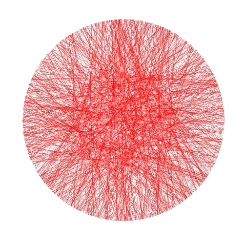
Some students choose chords as the line between two random points on the circumference and conclude that the asked probability is around 1/3. This is the plot of one of their simulations, where 1000 random chords are chosen according this method and those longer than the side of the equilateral triangle are red coloured (smalller in grey):

Bertrand1

Some others choose a random radius and a random point in it. The chord then is the perpendicular through this point. They calculate that the asked probability is around 1/2:

Bertrand2

And some others choose a random point inside the circle and define the chord as the only one with this point as midpoint. For them, the asked probability is around 1/4:

Bertrand3

Who is right? Professor Bertrand knows that everybody is. In fact, his main purpose was to show how important is to define problems properly. Actually, he used this to give an unforgettable lesson to his students.

library(ggplot2)
n=1000
opt=theme(legend.position="none",
          panel.background = element_rect(fill="white"),
          panel.grid = element_blank(),
          axis.ticks=element_blank(),
          axis.title=element_blank(),
          axis.text =element_blank())
#First approach
angle=runif(2*n, min = 0, max = 2*pi)
pt1=data.frame(x=cos(angle), y=sin(angle))
df1=cbind(pt1[1:n,], pt1[((n+1):(2*n)),])
colnames(df1)=c("x1", "y1", "x2", "y2")
df1$length=sqrt((df1$x1-df1$x2)^2+(df1$y1-df1$y2)^2)
p1=ggplot(df1) + geom_segment(aes(x = x1, y = y1, xend = x2, yend = y2, colour=length>sqrt(3)), alpha=.4, lwd=.6)+
  scale_colour_manual(values = c("gray75", "red"))+opt
#Second approach
angle=2*pi*runif(n)
pt2=data.frame(aa=cos(angle), bb=sin(angle))
pt2$x0=pt2$aa*runif(n)
pt2$y0=pt2$x0*(pt2$bb/pt2$aa)
pt2$a=1+(pt2$x0^2/pt2$y0^2)
pt2$b=-2*(pt2$x0/pt2$y0)*(pt2$y0+(pt2$x0^2/pt2$y0))
pt2$c=(pt2$y0+(pt2$x0^2/pt2$y0))^2-1
pt2$x1=(-pt2$b+sqrt(pt2$b^2-4*pt2$a*pt2$c))/(2*pt2$a)
pt2$y1=-pt2$x0/pt2$y0*pt2$x1+(pt2$y0+(pt2$x0^2/pt2$y0))
pt2$x2=(-pt2$b-sqrt(pt2$b^2-4*pt2$a*pt2$c))/(2*pt2$a)
pt2$y2=-pt2$x0/pt2$y0*pt2$x2+(pt2$y0+(pt2$x0^2/pt2$y0))
df2=pt2[,c(8:11)]
df2$length=sqrt((df2$x1-df2$x2)^2+(df2$y1-df2$y2)^2)
p2=ggplot(df2) + geom_segment(aes(x = x1, y = y1, xend = x2, yend = y2, colour=length>sqrt(3)), alpha=.4, lwd=.6)+
scale_colour_manual(values = c("gray75", "red"))+opt
#Third approach
angle=2*pi*runif(n)
radius=runif(n)
pt3=data.frame(x0=sqrt(radius)*cos(angle), y0=sqrt(radius)*sin(angle))
pt3$a=1+(pt3$x0^2/pt3$y0^2)
pt3$b=-2*(pt3$x0/pt3$y0)*(pt3$y0+(pt3$x0^2/pt3$y0))
pt3$c=(pt3$y0+(pt3$x0^2/pt3$y0))^2-1
pt3$x1=(-pt3$b+sqrt(pt3$b^2-4*pt3$a*pt3$c))/(2*pt3$a)
pt3$y1=-pt3$x0/pt3$y0*pt3$x1+(pt3$y0+(pt3$x0^2/pt3$y0))
pt3$x2=(-pt3$b-sqrt(pt3$b^2-4*pt3$a*pt3$c))/(2*pt3$a)
pt3$y2=-pt3$x0/pt3$y0*pt3$x2+(pt3$y0+(pt3$x0^2/pt3$y0))
df3=pt3[,c(6:9)]
df3$length=sqrt((df3$x1-df3$x2)^2+(df3$y1-df3$y2)^2)
p3=ggplot(df3) + geom_segment(aes(x = x1, y = y1, xend = x2, yend = y2, colour=length>sqrt(3)), alpha=.4, lwd=.6)+scale_colour_manual(values = c("gray75", "red"))+opt

The Awesome Parrondo’s Paradox

A technique succeeds in mathematical physics, not by a clever trick, or a happy accident, but because it expresses some aspect of physical truth (O. G. Sutton)

Imagine three unbalanced coins:

  • Coin 1: Probability of head=0.495 and probability of tail=0.505
  • Coin 2: Probability of head=0.745 and probability of tail=0.255
  • Coin 3: Probability of head=0.095 and probability of tail=0.905

Now let’s define two games using these coins:

  • Game A: You toss coin 1 and if it comes up head you receive 1€ but if not, you lose 1€
  • Game B: If your present capital is a multiple of 3, you toss coin 2. If not, you toss coin 3. In both cases, you receive 1€ if coin comes up head and lose 1€ if not.

Played separately, both games are quite unfavorable. Now let’s define Game A+B in which you toss a balanced coin and if it comes up head, you play Game A and play Game B otherwise. In other words, in Game A+B you decide between playing Game A or Game B randomly.

Starting with 0€, it is easy to simulate the three games along 500 plays. This is an example of one of these simulations:#Rstats #R

Resulting profit of Game A+B after 500 plays  is +52€ and is -9€ and -3€ for Games A and B respectively. Let’s do some more simulations (I removed legends and titles but colors of games are the same):

#Rstats #R

As you can see, Game A+B is the most profitable in almost all the previous simulations. Coincidence? Not at all. This is a consequence of the stunning Parrondo’s Paradox which states that two losing games can combine into a winning one.

If you still don’t believe in this brain-crashing paradox, following you can see the empirical distributions of final profits of three games after 1.000 plays:#Rstats #R

After 1000 plays, mean profit of Game A is -13€, is -7€ for Game B and 17€ for Game A+B.

This paradox was discovered in the last nineties by the Spanish physicist Juan Parrondo and can help to explain, among other things, why investing in losing shares can result in obtaining big profits. Amazing:

require(ggplot2)
require(scales)
library(gridExtra)
opts=theme(
  legend.position = "bottom",
  legend.background = element_rect(colour = "black"),
  panel.background = element_rect(fill="gray98"),
  panel.border = element_rect(colour="black", fill=NA),
  axis.line = element_line(size = 0.5, colour = "black"),
  axis.ticks = element_line(colour="black"),
  panel.grid.major = element_line(colour="gray75", linetype = 2),
  panel.grid.minor = element_blank(),
  axis.text.y = element_text(colour="gray25", size=15),
  axis.text.x = element_text(colour="gray25", size=15),
  text = element_text(size=20),
  plot.title = element_text(size = 35))
PlayGameA = function(profit, x, c) {if (runif(1) < c-x) profit+1 else profit-1}
PlayGameB = function(profit, x1, c1, x2, c2) {if (profit%%3>0) PlayGameA(profit, x=x1, c=c1) else PlayGameA(profit, x=x2, c=c2)}
####################################################################
#EVOLUTION
####################################################################
noplays=500
alpha=0.005
profit0=0
results=data.frame(Play=0, ProfitA=profit0, ProfitB=profit0, ProfitAB=profit0)
for (i in 1:noplays) {results=rbind(results, c(i,
    PlayGameA(profit=results[results$Play==(i-1),2], x =alpha, c =0.5),
    PlayGameB(profit=results[results$Play==(i-1),3], x1=alpha, c1=0.75, x2=alpha, c2=0.1),
    if (runif(1)<0.5) PlayGameA(profit=results[results$Play==(i-1),4], x =alpha, c =0.5) else PlayGameB(profit=results[results$Play==(i-1),4], x1=alpha, c1=0.75, x2=alpha, c2=0.1)
    ))}
results=rbind(data.frame(Play=results$Play, Game="A",   Profit=results$ProfitA),
              data.frame(Play=results$Play, Game="B",   Profit=results$ProfitB),
              data.frame(Play=results$Play, Game="A+B", Profit=results$ProfitAB))
ggplot(results, aes(Profit, x=Play, y=Profit, color = Game)) +
  scale_x_continuous(limits=c(0,noplays), "Plays")+
  scale_y_continuous(limits=c(-75,75), expand = c(0, 0), "Profit")+
  labs(title="Evolution of profit games along 500 plays")+
  geom_line(size=3)+opts
####################################################################
#DISTRIBUTION
####################################################################
noplays=1000
alpha=0.005
profit0=0
results2=data.frame(Play=numeric(0), ProfitA=numeric(0), ProfitB=numeric(0), ProfitAB=numeric(0))
for (j in 1:100) {results=data.frame(Play=0, ProfitA=profit0, ProfitB=profit0, ProfitAB=profit0)
  for (i in 1:noplays) {results=rbind(results, c(i,
      PlayGameA(profit=results[results$Play==(i-1),2], x =alpha, c =0.5),
      PlayGameB(profit=results[results$Play==(i-1),3], x1=alpha, c1=0.75, x2=alpha, c2=0.1),
      if (runif(1)<0.5) PlayGameA(profit=results[results$Play==(i-1),4], x =alpha, c =0.5)
      else PlayGameB(profit=results[results$Play==(i-1),4], x1=alpha, c1=0.75, x2=alpha, c2=0.1)))}
      results2=rbind(results2, results[results$Play==noplays, ])}
results2=rbind(data.frame(Game="A", Profit=results2$ProfitA),
data.frame(Game="B", Profit=results2$ProfitB),
data.frame(Game="A+B", Profit=results2$ProfitAB))
ggplot(results2, aes(Profit, fill = Game)) +
  scale_x_continuous(limits=c(-150,150), "Profit")+
  scale_y_continuous(limits=c(0,0.02), expand = c(0, 0), "Density", labels = percent)+
  labs(title=paste("Parrondo's Paradox (",as.character(noplays)," plays)",sep=""))+
  geom_density(alpha=.75)+opts