Why I Think Atletico De Madrid Will Win 2013/14 Spanish Liga Of Football

Prediction is difficult, especially of the future (Mark Twain)

Let me start with two important premises. First of all, I am not into football so I do not support any team. Second, this post is just an opinion based on mathematics but football, as all of you know, is not an exact science. Football is football.

This is a good moment to analyse Spanish Liga of football. F. C. Barcelona and Atletico de Madrid share first place of the championship followed closely by Real Madrid. But analysing results over the time can give us an interesting insight about capabilities of top three teams.

I have run a Bradley-Terry model for pairwise comparisons. The Bradley-Terry model deals with a situation in which n individuals or items are compared to one another in paired contests. In my case the model uses confrontations and its results as input. The Bradley-Terry model (Bradley and Terry 1952) assumes that in a contest between any two players, say player i and player j, the odds that i beats j are xi/xj, where xi and xj are positive-valued parameters which might be thought of as representing ability.

Time plays a key role in my analysis. This is what happens when you estimate abilities of top three teams over the time:

abilities

After 20 rounds, Atletico de Madrid and Barcelona have the same estimated ability but while Barcelona is continuosly losing ability since the beginning, Atletico de Madrid presents a robust or even growing evolution. Of course, it depends on how both teams begun the championship. The higher you start, the more you can lose; but watching this graph I can not help feeling that Atletico de Madrid keep their morale higher than Barcelona.

Another interesting output of  the Bradley-Terry model are estimated probabilites of beating teams each others. Since these probabilities depends on previous abilities, Barcelona and Atletico de Madrid have same chances of winning a hypothetical match. But once again, evolution of these probabilities can change our perception:

probabilities

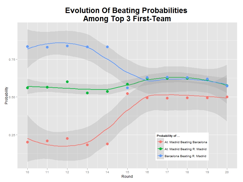
As you can see, Atletico de Madrid has increased the probability of beating Barcelona from 0.25 to 0.50 in just one round and Barcelona has lost more than this probability in the same time. Once again, it seems that Atletico de Madrid is increasingly confidence time by time. And confidence is important in this game. Luckily, football is unpredictable but after taking time into account I dare to say that Atletico de Madrid will win the championship. I am pretty sure.

Here you have the code I wrote for the analysis. Maybe you would like to make your own predictions:

library("BradleyTerry2")
library("xlsx")
library("ggplot2")
library("reshape")
football <-read.xlsx("CalendarioLiga2013-14 2.xls", sheetName= "results", header=TRUE)
inv_logit <- function(p) {exp(p) / (1 + exp(p))}
prob_BT   <- function(ability_1, ability_2) {inv_logit(ability_1 - ability_2)}
rounds <- sort(unique(football$round))
# Initialization
football.pts.ev <- as.data.frame(c())
football.abl.ev <- as.data.frame(c())
football.prb.ev <- as.data.frame(c())
# Points evolution: football.pts.ev
for (i in 1:length(rounds))
{
  football.home <-aggregate( home.wins ~ home.team, data=football[football$round<=rounds[i],], FUN=sum)
  colnames(football.home) <- c('Team', 'Points')
  football.away <-aggregate( away.wins ~ away.team, data=football[football$round<=rounds[i],], FUN=sum)
  colnames(football.away) <- c('Team', 'Points')
  football.all <-rbind(football.home,football.away)
  football.points <-aggregate( Points ~ Team, data=football.all, FUN=sum)
  football.points$round<-rounds[i]
  football.pts.ev <- rbind(football.points, football.pts.ev)
}
# BT Models 
# Abilities and probabilities evolution: football.abl.ev and football.prb.ev
# We start from 6th. round to have good information
for (i in 6:length(rounds))
{
  footballBTModel      <- BTm(cbind(home.wins, away.wins), home.team, away.team, data = football[football$round<=rounds[i],], id = "team")
  team_abilities       <- data.frame(BTabilities(footballBTModel))$ability 
  names(team_abilities) <-unlist(attr(BTabilities(footballBTModel), "dimnames")[1][1])
  team_probs           <- outer(team_abilities, team_abilities, prob_BT) 
  diag(team_probs)     <- 0 
  team_probs           <- melt(team_probs)
  colnames(team_probs) <- c('team', 'adversary', 'probability')
  team_probs$round<-rounds[i]
  football.prb.ev <- rbind(team_probs, football.prb.ev)
  football.abl.ev.df <- data.frame(rownames(data.frame(BTabilities(footballBTModel))),BTabilities(footballBTModel))
  football.abl.ev.df$round<-rounds[i]
  colnames(football.abl.ev.df) <- c('team', 'ability', 's.e.', 'round')
  football.abl.ev <- rbind(football.abl.ev.df, football.abl.ev)
}
# Probabilities of top 3 teams
football.prb.ev.3 <- football.prb.ev[
    ((football.prb.ev$team == "At. Madrid" & football.prb.ev$adversary == "R. Madrid")|
     (football.prb.ev$team == "At. Madrid" & football.prb.ev$adversary == "Barcelona")|
     (football.prb.ev$team == "Barcelona"  & football.prb.ev$adversary == "R. Madrid"))&
      football.prb.ev$round>=10, ]
football.prb.ev.3$teambyadver <- interaction(football.prb.ev.3$team, football.prb.ev.3$adversary, sep = " Beating ")
# Abilities of top 3 teams
football.abl.ev.3 <- football.abl.ev[(football.abl.ev$team == "At. Madrid" | 
                                     football.abl.ev$team == "R. Madrid"  | 
                                     football.abl.ev$team == "Barcelona")&
                                     football.abl.ev$round>=10, ]
ggplot(data = football.prb.ev.3, aes(x = round, y = probability, colour = teambyadver)) +  
  stat_smooth(method = "loess", formula = y ~ x, size = 1, alpha = 0.25)+
  geom_point(size = 4) +
  theme(legend.position = c(.75, .15))+
  labs(list(x = "Round", y = "Probability"))+
  labs(colour = "Probability of ...")+
  ggtitle("Evolution Of Beating Probabilities \nAmong Top 3 First-Team") + 
  theme(plot.title = element_text(size=25, face="bold"))+
  scale_x_continuous(breaks = c(10,11,12,13,14,15,16,17,18,19,20))
ggplot(data = football.abl.ev.3, aes(x = round, y = ability, colour = team)) +  
  stat_smooth(method = "loess", formula = y ~ x, size = 1, alpha = 0.25)+
  geom_point(size = 4) +
  theme(legend.position = c(.75, .75))+
  labs(list(x = "Round", y = "Ability"))+
  labs(colour = "Ability of ...")+
  ggtitle("Evolution Of Abilities \nOf Top 3 First-Team") + 
  theme(plot.title = element_text(size=25, face="bold"))+
  scale_x_continuous(breaks = c(10,11,12,13,14,15,16,17,18,19,20))

Cellular Automata: The Beauty Of Simplicity

I am strangely attracted to you (Cole Porter)

Imagine a linear grid that extends to the left and right. The grid consists of cells that may be only one of these two states: On or Off. At each time step, the next state of a cell is computed as a function of its left and right neighbors and the current state of the cell itself. Given one cell, if the three cells (both inmediate neighbors and cell itself) are on or off, next state of the cell is Off. Otherwise, next state is On. These simple rules can be represented graphically as follows, where white colour is equal to Off and black one is equal to On:

rules5

Lets assume that time flows in a downward direction; thus, the cell inmediately below another cell represents the next sate. Last assumption: cells on one edge are neighbors of the cells of the opposite edge. Whe have defined a One-Dimensional Cellular Automata with finite states.

This is what happens when we initialize as Off all cells except for the two center cells, initialized as On:

triangle3A2 triangle4A2 triangle5A2triangle6A2

Previous plots represent time evolution of the automata for 8, 16, 32 and 64 degress of time (i.e. depth). And this is the result for 256 degrees:

triangle8A2

Result is very similar to the well known Sierpinski triangle. And this is what happens when you initialize cells ramdomly:

chaos8A2
I like a lot the small triangles that appears as automata evolves. I am strangely attracted to them.

Here you have the code to build triangle:

library(sp)
width <-2^5
depth <-width/2
gt = GridTopology(cellcentre=c(1,1),cellsize=c(1,1),cells=c(width, depth))
gt = SpatialGrid(gt)
z <- data.frame(status=sample(0:0, width, replace=T))
z[width/2, 1] <- 1
z[width/2+1, 1] <- 1
for (i in (width+1):(width*depth))
{
  ilf <- i-width-1
  iup <- i-width
  irg <- i-width+1
  if (i%%width==0) irg <- i-2*width+1
  if (i%%width==1) ilf <- i-1
  if((z[ilf,1]+z[iup,1]+z[irg,1]>0)&(z[ilf,1]+z[iup,1]+z[irg,1]<3))
  {st <- 1} else {st <- 0}
  nr<-as.data.frame(st)
  colnames(nr)<-c("status")
  z<-rbind(z,nr)
}
sgdf = SpatialGridDataFrame(gt, z)
image(sgdf, col=c("white", "black"))

I Need A New Computer To Draw Fractals!

Computer Science is no more about computers than astronomy is about telescopes (E. W. Dijkstra)

Some days ago I published a post about how to build fractals with R using Multiple Reduction Copt Machine (MRCM) algorithm. Is that case I used a feature of the grid package that allows you to locate objects easily into the viewPort avoiding to work with coordinates. It does not work well if you want to divide your seed image into five subimages located in the vertex of a regular pentagon. No problem: after refreshing some trigonometric formulas and after understanding how to work with coordinates I felt strong enough to program the Final-MRCM-Fractal-Builder. But here comes the harsh reality. My computer crashes when I try to go beyond five degrees of depth. Imposible. In the example of Sierpinski’s triangle, where every square in divided into three small ones, I reached seven degrees of depth. I am deeply frustrated. These are drawings for 1, 2, 3 and 5 degrees of depth.

Rplot01c Rplot02c Rplot03cRplot05c

Please, if someone modifies code to make it more efficient, let me know. I used circles in this case instead squares. Here you have it:

library(grid)
grid.newpage()
rm(list = ls())
ratio <- 0.4
pmax <- 5 # Depth
vp1 <- viewport(w=1, h=1)
vp2 <- viewport(w=ratio, h=ratio, just=c(0.75*sin(2*pi*1/5)+0.5, 0.75*cos(2*pi*1/5)+0.75*pi*1/5))
vp3 <- viewport(w=ratio, h=ratio, just=c(0.75*sin(2*pi*0/5)+0.5, 0.75*cos(2*pi*0/5)+0.75*pi*1/5))
vp4 <- viewport(w=ratio, h=ratio, just=c(0.75*sin(2*pi*2/5)+0.5, 0.75*cos(2*pi*2/5)+0.75*pi*1/5))
vp5 <- viewport(w=ratio, h=ratio, just=c(0.75*sin(2*pi*3/5)+0.5, 0.75*cos(2*pi*3/5)+0.75*pi*1/5))
vp6 <- viewport(w=ratio, h=ratio, just=c(0.75*sin(2*pi*4/5)+0.5, 0.75*cos(2*pi*4/5)+0.75*pi*1/5))
pushViewport(vp1)
grid.rect(gp=gpar(fill="white", col=NA))
m <- as.matrix(expand.grid(rep(list(2:6), pmax)))
for (j in 1:nrow(m))
{
for(k in 1:ncol(m)) {pushViewport(get(paste("vp",m[j,k],sep="")))}
grid.circle(gp=gpar(col="dark grey", lty="solid", fill=rgb(sample(0:255, 1),sample(0:255, 1),sample(0:255, 1), alpha= 95, max=255)))
upViewport(pmax)
}

What The Hell Is Pi Doing Here?

Nothing in Nature is random … A thing appears random only through the incompleteness of our knowledge (Benedict Spinoza)

This is one of my favorite mathematical mysteries. In 1991 David Boll was trying to confirm that the neck of the Mandelbrot Set is 0 in thickness. Neck is located at -0.75+0i (where two biggest circles meet each other). Mandelbrot50He tried with complex numbers like -0.75+εi for small values of ε demonstrating the divergence of all these numbers. And here comes the mystery: multiplying ε and the corresponding number of iterations it took for the iterate to diverge, gives an approximation of π that is within ±ε. Is not fascinating? I replicated David Boll’s experiment for positive and negative values of ε. I draw results as follows:

mandelbrot

Before doing it, I thought I was going to find some pattern in the graphic. Apart from the mirror effect produced by the sign of ε, there is nothing recognizable. Convergence is chaotic. Here you have the code. This example is also nice to practice with ggplot2 package, one of the totems of R:

i<-0    # Counter of iterations
x  <- 0 # Initialization
while (Mod(x) <= 2)
{
x <- x^2+(c+complex(real = 0, imaginary = e))
i <- i+1
}
i
}
results <- as.data.frame(c(NULL,NULL))
for (j in 1:length(epsilons))
{results <- rbind(results, c(epsilons[j], testMSConvergence(epsilons[j])))}
colnames(results) <- c('epsilon', 'iterations')
dev.off()
p <- ggplot(results, aes(epsilon,abs(epsilon)*iterations))+
xlab("epsilon")+
ylab("abs(epsilon)*iterations")+
opts(axis.title.x=theme_text(size=16)) +
opts(axis.title.y=theme_text(size=16)) +
ggtitle("How to Estimate Pi Using Mandelbrot Set's Neck")+
theme(plot.title = element_text(size=20, face="bold"))
p <- p + geom_ribbon(data=results,aes(ymin=abs(epsilon)*iterations-abs(epsilon),ymax=abs(epsilon)*iterations+abs(epsilon)), alpha=0.3)
p <- p + geom_abline(intercept = pi, , slope = 0, size = 0.4, linetype=2, colour = "black", alpha=0.8)
p <- p + geom_line(colour = "dark blue", size = 1, linetype = 1)
p <- p + geom_text(x = 0, y = pi, label="pi", vjust=2, colour="dark blue")
p <- p + geom_point(x = 0, y = pi, size = 6, colour="dark blue")
p + geom_point(x = 0, y = pi, size = 4, colour="white")

Building Affine Transformation Fractals With R

Clouds are not spheres, mountains are not cones, coastlines are not circles and bark is not smooth, nor does lightning travel in a straight line (Benoit Maldelbrot)

Fractals are beautiful, hypnotics, mysterious. Cantor set has as many points as the real number line but has zero measure. After 100 steps, the Koch curve created from a 1 inch segment is long enough  to wrap around the Earth at the equator nearly four thousand times. The Peano Curve is a line that has the same dimension as a plane. Fractals are weird mathematical objects. Fractals are very cool.

One way to build fractals is using the Multiple Reduction Copy Machine (MRCM) algorithm which uses affine linear transformations over a seed image to build fractals. MRCM are iterative algorithms that perform some sort of copy+paste task. The idea is quite simple: take a seed image, transform it (clonation, scalation, rotation), obtain the new image and iterate.

To create the Sierpinsky Gasket Fractal you part from a square. Then you divide it into three smaller squares, locate them as a pyramid and iterate doing the same with avery new square created. Making these things is very easy with grid package. Defining the division (i.e. the affine transformation) properly using viewPort function and navigating between them is all you need. Here you have the Sierpinsky Gasket Fractal with 1, 3, 5 and 7 levels of depth. I filled in squares with random colours (I like giving some touch of randomness to pictures). Here you have pictures:

Rplot01 Rplot03

Rplot05 Rplot07

And here you have the code. Feel free to build your own fractals.

library(grid)
rm(list = ls())
grid.newpage()
pmax <- 5 # Depth of the fractal
vp1=viewport(x=0.5,y=0.5,w=1, h=1)
vp2=viewport(w=0.5, h=0.5, just=c("centre", "bottom"))
vp3=viewport(w=0.5, h=0.5, just=c("left", "top"))
vp4=viewport(w=0.5, h=0.5, just=c("right", "top"))
pushViewport(vp1)
m <- as.matrix(expand.grid(rep(list(2:4), pmax)))
for (j in 1:nrow(m))
{
for(k in 1:ncol(m)) {pushViewport(get(paste("vp",m[j,k],sep="")))}
grid.rect(gp=gpar(col="dark grey", lty="solid",
fill=rgb(sample(0:255, 1),sample(0:255, 1),sample(0:255, 1), alpha= 95, max=255)))
upViewport(pmax)
}