Tag Archives: music

The Somnambulist and Pi

How wary we are of something warm and unborn. Something calmly by zero will divide (Unbegotten, The Somnambulist)

Some time ago, I assumed the mission to draw a plot for the cover of the new album of The Somnambulist, a music band from Berlin. They wanted a circlization of Pi, which is a graphic where numbers are represented in a circular layout. The idea is connecting each digit of Pi to its successive digit with links to the position of the numerically corresponding external sectors. I used a color palette composed by 10 nuances of the visible spectrum as a tribute for Planck, as Marco (the vocalist) requested me. After a number of attempts:

somnambulist

The album is named Unbegotten, a german word which means archaic. As Marco told me, in theology it also means kind of eternal because of being never born and so never dying. I like how π is integrated into the title to substitute the string “tt” in the middle. Pi is also eternal so the association is genuine.

The music of The Somnambulist is intense, dark and powerful and is waiting for you here to listen it. My favorite song is the one that gives name to the album.

If you want to know more about circlizong numbers, you can visit this post, where you also can see the code I used as starting point to do this plot.

A Visualization Of The 100 Greatest Love Songs ft. D3.js

What would you do? If my heart was torn in two (More Than Words, Extreme)

Playing with rCharts package I had the idea of representing the list of 100 best love songs as a connected set of points which forms a heart. Songs can be seen putting mouse cursor over each dot:

You can reproduce it with this simple code:

library(dplyr)
library(rCharts)
library(rvest)
setwd("YOUR WORKING DIRECTORY HERE")
heart <- function(r,x) {ifelse(abs(x)<2, ifelse(r%%2==0, sqrt(1-(abs(x)-1)^2), acos(1-abs(x))-pi), 0)} data.frame(x=seq(from=-3, to=3, length.out=100)) %>% 
  mutate(y=jitter(heart(row_number(), x), amount=.1)) -> df
love_songs <- html("http://www.cs.ubc.ca/~davet/music/list/Best13.html") love_songs %>%
  html_nodes("table") %>%
  .[[2]] %>%
  html_table(header=TRUE, fill = TRUE) %>%
  cbind(df) -> df
m1=mPlot(x = "x",  y = "y",  data = df,  type = "Line")
m1$set(pointSize = 5, 
       lineColors = c('red', 'red'),
       width = 850,
       height = 600,
       lineWidth = 2,
       hoverCallback = "#! function(index, options, content){
       var row = options.data[index]
       return '<b>' + row.ARTIST + '</b>' + '<br/>' + row.TITLE} !#",
       grid=FALSE,
       axes=FALSE)
m1$save('Top_100_Greatest_Love_Songs.html', standalone = TRUE)

Discovering Shiny

It is not an experiment if you know it is going to work (Jeff Bezos)

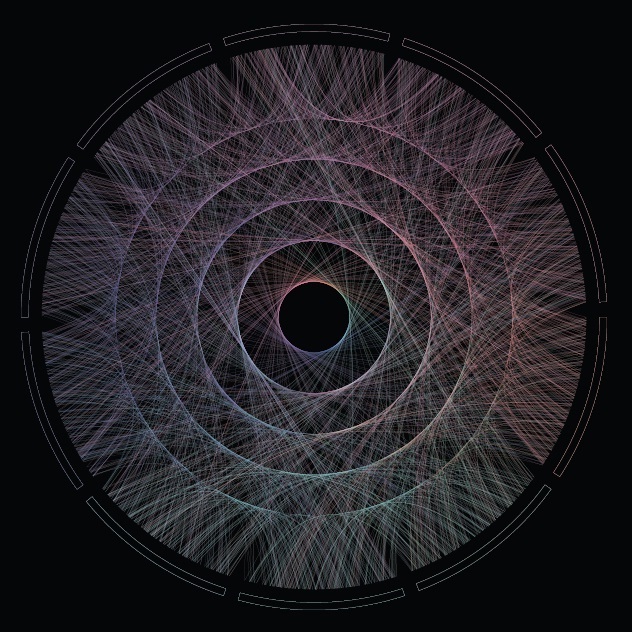
From time to time, I discover some of my experiments translated into Shiny Apps, like this one. Some days ago, I discovered one of these translations and I contacted the author, who was a guy from Vietnam called Vu Anh. I asked him to do a Shiny App from this experiment. Vu was enthusiastic with the idea. We defined some parameters to play with shape, number, width and alpha of lines as well as background color and I received a perfect release of the application in just a few hours. With just a handful of parameters, possible outputs are almost infinite. Following you can find some of them:

SinyCollageI think the code is a nice example to take the first steps in Shiny. If you are not used to Markdown files, you can follow this instructions to run the code.

Vu is a talented guy, who loves maths and programming. He represents the future of our nice profession and I predict a successful future for him. Do not miss his brand new blog. I am sure you will find amazing things there.

This is the code of the app:

---
title: "Maths, Music and Merkbar"
author: "Brother Rain"
date: "18/03/2015"
output: html_document
runtime: shiny
---
 
## Load Data
 
```{r}
library(circlize)
library(scales)
factors = as.factor(0:9)
lines = 2000 #Number of lines to plot in the graph
alpha = 0.4  #Alpha for color lines
colors0=c(
    rgb(239,143,121, max=255),
    rgb(126,240,188, max=255),
    rgb(111,228,235, max=255),
    rgb(127,209,249, max=255),
    rgb( 74,106,181, max=255),
    rgb(114,100,188, max=255),
    rgb(181,116,234, max=255),
    rgb(226,135,228, max=255),
    rgb(239,136,192, max=255),
    rgb(233,134,152, max=255)
)
# You can find the txt file here:
# http://www.goldennumber.net/wp-content/uploads/2012/06/Phi-To-100000-Places.txt
phi=readLines("data/Phi-To-100000-Places.txt")[5]
```
 
## Visualization
 
```{r, echo=FALSE}
fluidPage(
  fluidRow(
    column(width = 4,
        sidebarPanel(
            sliderInput("lines", "Number of lines:", min=100, max=100000, step=100, value=500), 
            sliderInput("alpha", "Alpha:", min=0.01, max=1, step=0.01, value=0.4),
            sliderInput("lwd", "Line width", min=0, max=1, step=0.05, value=0.2),
            selectInput("background", "Background:",
                c("Purple" = "mediumpurple4", "Gray" = "gray25", "Orange"="orangered4", 
                  "Red" = "red4", "Brown"="saddlebrown", "Blue"="slateblue4", 
                  "Violet"="palevioletred4", "Green"="forestgreen", "Pink"="deeppink"), selected="Purple"),
            sliderInput("h0", "h0:", min=0, max=0.4,
                    step=0.0005, value=0.1375),
           sliderInput("h1", "h1:", min=0, max=0.4,
                step=0.0005, value=0.1125),
            width=12
        )
    ),
    column(width = 8,
        renderPlot({
            # get data
            phi=gsub("\\.","", substr(phi,1,input$lines))
            phi=gsub("\\.","", phi)
            position=1/(nchar(phi)-1)
             
            # create circos
            circos.clear()
            par(mar = c(1, 1, 1, 1), lwd = 0.1,
                cex = 0.7, bg=alpha(input$background, 1))
            circos.par(
                "cell.padding"=c(0.01,0.01),
                "track.height" = 0.025,
                "gap.degree" = 3
            )
            circos.initialize(factors = factors, xlim = c(0, 1))
            circos.trackPlotRegion(factors = factors, ylim = c(0, 1))
            ## create first region
            for (i in 0:9) {
                circos.updatePlotRegion(
                    sector.index = as.character(i),
                    bg.col = alpha(input$background, 1),
                    bg.border=alpha(colors0[i+1], 1)
                )
            }
            for (i in 1:(nchar(phi)-1)) {
                m=min(as.numeric(substr(phi, i, i)), as.numeric(substr(phi, i+1, i+1)))
                M=max(as.numeric(substr(phi, i, i)), as.numeric(substr(phi, i+1, i+1)))
                d=min((M-m),((m+10)-M))
                col=t(col2rgb(colors0[(as.numeric(substr(phi, i, i))+1)]))
                for(index in 1:3){
                    col[index] = max(min(255, col[index]), 0)
                }
                if (d>0) {
                    circos.link(
                        substr(phi, i, i), position*(i-1),
                        substr(phi, i+1, i+1), position*i,
                        h = input$h0 * d + input$h1,
                        lwd=input$lwd,
                        col=alpha(rgb(col, max=255), input$alpha), rou = 0.92
                    )
                }
            }
            }, width=600, height=600, res=192)
    )
  )
)
 
 
```

Maths, Music and Merkbar

Control is what we already know. Control is where we have already ventured. Control is what helps us predict the future. (Merkbar)

Maths and music get along very well. Last December I received a mail from a guy called Jesper. He is one of the two members of Merkbar: a electronic music band from Denmark. As can be read in their website:

Merkbar is Jesper and David who are both interested in the psychedelic worlds and oriental spiritualism. They both studied Computer Music, where they’ve done research in sound synthesis, generative composition and the design of new digital instrument.

They asked me a front cover for their new album which will be released at the beginning of 2015. Why? Because they liked this post I did about circlizing numbers.  To do this plot I circlized the Golden Ratio number (Phi). But in this case I changed ribbons (all equal pairs of consecutive numbers gather together) by lines (every pair of consecutive numbers form a different line). As I did before, I used circlize package, which implements in R the features of Circos, a software to create stunning circular visualizations.

The final plot represents the first 2.000 digits of Phi:

Merkbar Cover2

You can hear an advancement of their new album here, which is called “Phi”. Enjoy their sensitive and full-of-shades music: you will be delightfully surprised as I was.

This is the code to circlize Phi:

library(circlize)
library(scales)
factors = as.factor(0:9)
lines = 2000 #Number of lines to plot in the graph
alpha = 0.4  #Alpha for color lines
colors0=c(rgb(239,143,121, max=255), rgb(126,240,188, max=255), rgb(111,228,235, max=255),
          rgb(127,209,249, max=255), rgb( 74,106,181, max=255), rgb(114,100,188, max=255),
          rgb(181,116,234, max=255), rgb(226,135,228, max=255), rgb(239,136,192, max=255),
          rgb(233,134,152, max=255))
#You can find the txt file here: http://www.goldennumber.net/wp-content/uploads/2012/06/Phi-To-100000-Places.txt
phi=readLines("Phi-To-100000-Places.txt")[5]
phi=gsub("\\.","", substr(phi,1,lines))
phi=gsub("\\.","", phi)
position=1/(nchar(phi)-1)
#This code generates a pdf file in your working directory
pdf(file="CirclizePhi.pdf", width=25, height=25)
circos.clear()
par(mar = c(1, 1, 1, 1), lwd = 0.1, cex = 0.7, bg=alpha("black", 1))
circos.par("cell.padding"=c(0.01,0.01), "track.height" = 0.025, "gap.degree" = 3)
circos.initialize(factors = factors, xlim = c(0, 1))
circos.trackPlotRegion(factors = factors, ylim = c(0, 1))
for (i in 0:9) {circos.updatePlotRegion(sector.index = as.character(i), bg.col = alpha("black", 1), bg.border=alpha(colors0[i+1], 1))}
for (i in 1:(nchar(phi)-1)) {
  m=min(as.numeric(substr(phi, i, i)), as.numeric(substr(phi, i+1, i+1)))
  M=max(as.numeric(substr(phi, i, i)), as.numeric(substr(phi, i+1, i+1)))
  d=min((M-m),((m+10)-M))
  col=t(col2rgb(colors0[(as.numeric(substr(phi, i, i))+1)]))
  if (col[1]>255) col[1]=255;if (col[2]>255) col[2]=255;if (col[3]>255) col[3]=255
  if (col[1]<0) col[1]=0;if (col[2]<0) col[2]=0;if (col[3]<0) col[3]=0 if (d>0) circos.link(substr(phi, i, i), position*(i-1), substr(phi, i+1, i+1), position*i, h = 0.1375*d+0.1125, lwd=0, col=alpha(rgb(col, max=255), alpha), rou = 0.92)
}
dev.off()

The Sound Of Mandelbrot Set

Music is the pleasure the human soul experiences from counting without being aware that it is counting (Gottfried Leibniz)

I like the concept of sonification: translating data into sounds. There is a huge amount of contents in the Internet about this technique and there are several packages in R to help you to sonificate your data. Maybe one of the most accessible is tuneR, the one I choosed for this experiment. Do not forget to have a look to playitbyr: a package that allows you to listen to a data.frame in R by mapping columns onto sonic parameters, creating an auditory graph, as you can find in its website. It has a very similar syntaxis to ggplot. I will try to post something about playitbyr in the future.

Let me start plotting the Mandelbrot Set. I know you have seen it lot of times but it is very easy to plot in with R and result is extremely beautiful. Here you have four images corresponding to 12, 13, 14 and 15 iterations of the set’s generator. I like a lot how the dark blue halo around the Set evaporates as number of iterations increases.

Mandelbrot12Mandelbrot13Mandelbrot14Mandelbrot15

And here you have the Set generated by 50 iterations. This is the main ingredient of the experiment:Mandelbrot50

Mandelbrot Set is generated by the recursive formula xt+1=xt2+c, with x0=0. A complex number c belongs to the Mandelbrot Set if its module after infinite iterations is finite. It is not possible to iterate a infinite number of times so every representation of Mandelbrot Set is just an approximation for a usually big amount of iterations. First image of Mandelbrot Set was generated in 1978 by Robert W. Brooks and Peter Matelski. You can find it here. I do not know how long it took to obtain it but you will spend only a couple of minutes to generate the ones you have seen before. It is amazing how computers have changed in this time!

This iterative equation is diabolical. To see just how pathological is, I transformed the succession of modules of xt generated by a given c in a succession of sounds. Since it is known that if one of this iterated complex numbers exceeds 2 in module then it is not in the Mandelbrot Set, frequencies of these sounds are bounded between 280 Hz (when module is equal to zero) and 1046 Hz (when module is equal or greater to 2). I called this function CreateSound. Besides the initial complex, you can choose how many notes and how long you want for your composition.

I tried with lot of numbers and results are funny. I want to stand out three examples from the rest:

  • -1+0i gives the sequence 0, −1, 0, −1, 0 … which is bounded. Translated into music it sounds like an ambulance siren.
  • -0.1528+1.0397i that is one of the generalized Feigenbaum points, around the Mandelbrot Set is conjetured to be self-similar. It sounds as a kind of Greek tonoi.
  • -3/4+0.01i which presents a crazy slow divergence. I wrote a post some weeks ago about this special numbers around the neck of Mandelbrot Set and its relationship with PI.

All examples are ten seconds length. Take care with the size of the WAV file when you increase duration. You can create your own music files with the code below. If you want to download my example files, you can do it here. If you discover something interesting, please let me know.

Enjoy the music of Mandelbrot:

# Load Libraries
library(ggplot2)
library(reshape)
library(tuneR)
rm(list=ls())
# Create a grid of complex numbers
c.points <- outer(seq(-2.5, 1, by = 0.002),1i*seq(-1.5, 1.5, by = 0.002),'+')
z <- 0
for (k in 1:50) z <- z^2+c.points # Iterations of fractal's formula
c.points <- data.frame(melt(c.points))
colnames(c.points) <- c("r.id", "c.id", "point")
z.points <- data.frame(melt(z))
colnames(z.points) <- c("r.id", "c.id", "z.point")
mandelbrot <- merge(c.points, z.points, by=c("r.id","c.id")) # Mandelbrot Set
# Plotting only finite-module numbers
ggplot(mandelbrot[is.finite(-abs(mandelbrot$z.point)), ], aes(Re(point), Im(point), fill=exp(-abs(z.point))))+
geom_tile()+theme(legend.position="none", axis.title.x = element_blank(), axis.title.y = element_blank())
#####################################################################################
# Function to translate numbers (complex modules) into sounds between 2 frequencies
#   the higher the module is, the lower the frequencie is
#   modules greater than 2 all have same frequencie equal to low.freq
#   module equal to 0 have high.freq
#####################################################################################
Module2Sound <- function (x, low.freq, high.freq)
  {
    if(x>2 | is.nan(x)) {low.freq} else {x*(low.freq-high.freq)/2+high.freq}
  } 
#####################################################################################
# Function to create wave. Parameters:
#    complex     : complex number to test
#    number.notes: number of notes to create (notes = iterations)
#    tot.duration.secs: Duration of the wave in seconds
#####################################################################################
CreateSound <- function(complex, number.notes, tot.duration.secs)
{
  dur <- tot.duration.secs/number.notes
  sep1 <- paste(", bit = 16, duration= ",dur, ", xunit = 'time'),sine(")
  sep2 <- paste(", bit = 16, duration =",dur,",  xunit = 'time'))")
  v.sounds <- c()
  z <- 0
  for (k in 1:number.notes) 
  {
    z <- z^2+complex
    v.sounds <- c(v.sounds, abs(z))
  }
  v.freqs <- as.vector(apply(data.frame(v.sounds), 1, FUN=Module2Sound, low.freq=280, high.freq=1046))
  eval(parse(text=paste("bind(sine(", paste(as.vector(v.freqs), collapse = sep1), sep2)))
}
sound1 <- CreateSound(-3/4+0.01i     , 400 , 10) # Slow Divergence
sound2 <- CreateSound(-0.1528+1.0397i, 30  , 10) # Feigenbaum Point
sound3 <- CreateSound(-1+0i          , 20  , 10) # Ambulance Siren
writeWave(sound1, 'SlowDivergence.wav')
writeWave(sound2, 'FeigenbaumPoint.wav')
writeWave(sound3, 'AmbulanceSiren.wav')