Sweet home Alabama, Where the skies are so blue; Sweet home Alabama, Lord, I’m coming home to you (Sweet home Alabama, Lynyrd Skynyrd)
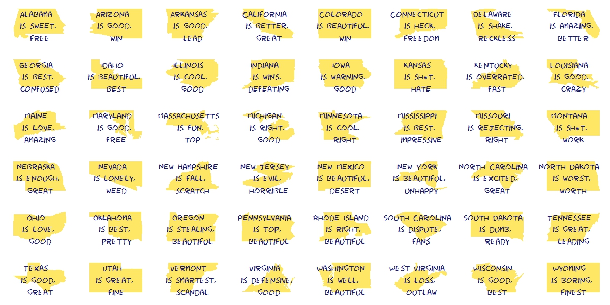
This is the second post I write to show the abilities of twitteR package and also the second post I write for KDnuggets. In this case my goal is to have an insight of what people tweet about american states. To do this, I look for tweets containing the exact phrase “[STATE NAME] is” for every states. Once I have the set of tweets for each state I do some simple text mining: cleaning, standardizing, removing empty words and crossing with these sentiment lexicons. Then I choose the two most common words to describe each state. You can read the original post here. This is the visualization I produced to show the result of the algorithm:

Since the right side of the map is a little bit messy, in the original post you can see a table with the couple of words describing each state. This is just an experiment to show how to use and combine some interesting tools of R. If you don’t like what Twitter says about your state, don’t take it too seriously.
This is the code I wrote for this experiment:
# Do this if you have not registered your R app in Twitter
library(twitteR)
library(RCurl)
setwd("YOUR-WORKING-DIRECTORY-HERE")
if (!file.exists('cacert.perm'))
{
  download.file(url = 'http://curl.haxx.se/ca/cacert.pem', destfile='cacert.perm')
}
requestURL="https://api.twitter.com/oauth/request_token"
accessURL="https://api.twitter.com/oauth/access_token"
authURL="https://api.twitter.com/oauth/authorize"
consumerKey = "YOUR-CONSUMER_KEY-HERE"
consumerSecret = "YOUR-CONSUMER-SECRET-HERE"
Cred <- OAuthFactory$new(consumerKey=consumerKey,
                         consumerSecret=consumerSecret,
                         requestURL=requestURL,
                         accessURL=accessURL,
                         authURL=authURL)
Cred$handshake(cainfo=system.file("CurlSSL", "cacert.pem", package="RCurl"))
save(Cred, file="twitter authentification.Rdata")
# Start here if you have already your twitter authentification.Rdata file
library(twitteR)
library(RCurl)
library(XML)
load("twitter authentification.Rdata")
registerTwitterOAuth(Cred)
options(RCurlOptions = list(cainfo = system.file("CurlSSL", "cacert.pem", package = "RCurl")))
#Read state names from wikipedia
webpage=getURL("http://simple.wikipedia.org/wiki/List_of_U.S._states")
table=readHTMLTable(webpage, which=1)
table=table[!(table$"State name" %in% c("Alaska", "Hawaii")), ]
#Extract tweets for each state
results=data.frame()
for (i in 1:nrow(table))
{
  tweets=searchTwitter(searchString=paste("'\"", table$"State name"[i], " is\"'",sep=""), n=200, lang="en")
  tweets.df=twListToDF(tweets)
  results=rbind(cbind(table$"State name"[i], tweets.df), results)
}
results=results[,c(1,2)]
colnames(results)=c("State", "Text")
library(tm)
#Lexicons
pos = scan('positive-words.txt',  what='character', comment.char=';')
neg = scan('negative-words.txt',  what='character', comment.char=';')
posneg=c(pos,neg)
results$Text=tolower(results$Text)
results$Text=gsub("[[:punct:]]", " ", results$Text)
# Extract most important words for each state
words=data.frame(Abbreviation=character(0), State=character(0), word1=character(0), word2=character(0), word3=character(0), word4=character(0))
for (i in 1:nrow(table))
{
  doc=subset(results, State==as.character(table$"State name"[i]))
  doc.vec=VectorSource(doc[,2])
  doc.corpus=Corpus(doc.vec)
  stopwords=c(stopwords("english"), tolower(unlist(strsplit(as.character(table$"State name"), " "))), "like")
  doc.corpus=tm_map(doc.corpus, removeWords, stopwords)
  TDM=TermDocumentMatrix(doc.corpus)
  TDM=TDM[Reduce(intersect, list(rownames(TDM),posneg)),]
  v=sort(rowSums(as.matrix(TDM)), decreasing=TRUE)
  words=rbind(words, data.frame(Abbreviation=as.character(table$"Abbreviation"[i]), State=as.character(table$"State name"[i]),
                                   word1=attr(head(v, 4),"names")[1],
                                   word2=attr(head(v, 4),"names")[2],
                                   word3=attr(head(v, 4),"names")[3],
                                   word4=attr(head(v, 4),"names")[4]))
}
# Visualization
require("sqldf")
statecoords=as.data.frame(cbind(x=state.center$x, y=state.center$y, abb=state.abb))
#To make names of right side readable
texts=sqldf("SELECT a.abb,
            CASE WHEN a.abb IN ('DE', 'NJ', 'RI', 'NH') THEN a.x+1.7
            WHEN a.abb IN ('CT', 'MA') THEN a.x-0.5  ELSE a.x END as x,
            CASE WHEN a.abb IN ('CT', 'VA', 'NY') THEN a.y-0.4 ELSE a.y END as y,
            b.word1, b.word2 FROM statecoords a INNER JOIN words b ON a.abb=b.Abbreviation")
texts$col=rgb(sample(0:150, nrow(texts)),sample(0:150, nrow(texts)),sample(0:150, nrow(texts)),max=255)
library(maps)
jpeg(filename = "States In Two Words v2.jpeg", width = 1200, height = 600, quality = 100)
map("state", interior = FALSE, col="gray40", fill=FALSE)
map("state", boundary = FALSE, col="gray", add = TRUE)
text(x=as.numeric(as.character(texts$x)), y=as.numeric(as.character(texts$y)), apply(texts[,4:5] , 1 , paste , collapse = "\n" ), cex=1, family="Humor Sans", col=texts$col)
dev.off()