Tag Archives: Twitter

Silhouettes

Romeo, Juliet, balcony in silhouette, makin o’s with her cigarette, it’s juliet (Flapper Girl, The Lumineers)

Two weeks ago I published this post for which designed two different visualizations. At the end, I decided to place words on the map of the United States. The discarded visualization was this other one, where I place the words over the silhouette of each state:

States In Two Words v1

I do not want to set aside this chart because I really like it and also because I think it is a nice example of the possibilities one have working with R.

Here you have the code. It substitutes the fragment of the code headed by “Visualization” of the original post:

library(ggplot2)
library(maps)
library(gridExtra)
library(extrafont)
opt=theme(legend.position="none",
             panel.background = element_blank(),
             panel.grid = element_blank(),
             axis.ticks=element_blank(),
             axis.title=element_blank(),
             axis.text =element_blank(),
             plot.title = element_text(size = 28))
vplayout=function(x, y) viewport(layout.pos.row = x, layout.pos.col = y)
grid.newpage()
jpeg(filename = "States In Two Words.jpeg", width = 1200, height = 600, quality = 100)
pushViewport(viewport(layout = grid.layout(6, 8)))
for (i in 1:nrow(table))
{
  wd=subset(words, State==as.character(table$"State name"[i]))
  p=ggplot() + geom_polygon( data=subset(map_data("state"), region==tolower(table$"State name"[i])), aes(x=long, y=lat, group = group), colour="white", fill="gold", alpha=0.6, linetype=0 )+opt
  print(p, vp = vplayout(floor((i-1)/8)+1, i%%8+(i%%8==0)*8))
  txt=paste(as.character(table$"State name"[i]),"\n is", wd$word1,"\n and", wd$word2, sep=" ")
  grid.text(txt, gp=gpar(font=1, fontsize=16, col="midnightblue", fontfamily="Humor Sans"), vp = viewport(layout.pos.row = floor((i-1)/8)+1, layout.pos.col = i%%8+(i%%8==0)*8))
}
dev.off()

The United States In Two Words

Sweet home Alabama, Where the skies are so blue; Sweet home Alabama, Lord, I’m coming home to you (Sweet home Alabama, Lynyrd Skynyrd)

This is the second post I write to show the abilities of twitteR package and also the second post I write for KDnuggets. In this case my goal is to have an insight of what people tweet about american states. To do this, I look for tweets containing the exact phrase “[STATE NAME] is” for every states. Once I have the set of tweets for each state I do some simple text mining: cleaning, standardizing, removing empty words and crossing with these sentiment lexicons. Then I choose the two most common words to describe each state. You can read the original post here. This is the visualization I produced to show the result of the algorithm:

States In Two Words v2

Since the right side of the map is a little bit messy, in the original post you can see a table with the couple of words describing each state. This is just an experiment to show how to use and combine some interesting tools of R. If you don’t like what Twitter says about your state, don’t take it too seriously.

This is the code I wrote for this experiment:

# Do this if you have not registered your R app in Twitter
library(twitteR)
library(RCurl)
setwd("YOUR-WORKING-DIRECTORY-HERE")
if (!file.exists('cacert.perm'))
{
  download.file(url = 'http://curl.haxx.se/ca/cacert.pem', destfile='cacert.perm')
}
requestURL="https://api.twitter.com/oauth/request_token"
accessURL="https://api.twitter.com/oauth/access_token"
authURL="https://api.twitter.com/oauth/authorize"
consumerKey = "YOUR-CONSUMER_KEY-HERE"
consumerSecret = "YOUR-CONSUMER-SECRET-HERE"
Cred <- OAuthFactory$new(consumerKey=consumerKey,
                         consumerSecret=consumerSecret,
                         requestURL=requestURL,
                         accessURL=accessURL,
                         authURL=authURL)
Cred$handshake(cainfo=system.file("CurlSSL", "cacert.pem", package="RCurl"))
save(Cred, file="twitter authentification.Rdata")
# Start here if you have already your twitter authentification.Rdata file
library(twitteR)
library(RCurl)
library(XML)
load("twitter authentification.Rdata")
registerTwitterOAuth(Cred)
options(RCurlOptions = list(cainfo = system.file("CurlSSL", "cacert.pem", package = "RCurl")))
#Read state names from wikipedia
webpage=getURL("http://simple.wikipedia.org/wiki/List_of_U.S._states")
table=readHTMLTable(webpage, which=1)
table=table[!(table$"State name" %in% c("Alaska", "Hawaii")), ]
#Extract tweets for each state
results=data.frame()
for (i in 1:nrow(table))
{
  tweets=searchTwitter(searchString=paste("'\"", table$"State name"[i], " is\"'",sep=""), n=200, lang="en")
  tweets.df=twListToDF(tweets)
  results=rbind(cbind(table$"State name"[i], tweets.df), results)
}
results=results[,c(1,2)]
colnames(results)=c("State", "Text")
library(tm)
#Lexicons
pos = scan('positive-words.txt',  what='character', comment.char=';')
neg = scan('negative-words.txt',  what='character', comment.char=';')
posneg=c(pos,neg)
results$Text=tolower(results$Text)
results$Text=gsub("[[:punct:]]", " ", results$Text)
# Extract most important words for each state
words=data.frame(Abbreviation=character(0), State=character(0), word1=character(0), word2=character(0), word3=character(0), word4=character(0))
for (i in 1:nrow(table))
{
  doc=subset(results, State==as.character(table$"State name"[i]))
  doc.vec=VectorSource(doc[,2])
  doc.corpus=Corpus(doc.vec)
  stopwords=c(stopwords("english"), tolower(unlist(strsplit(as.character(table$"State name"), " "))), "like")
  doc.corpus=tm_map(doc.corpus, removeWords, stopwords)
  TDM=TermDocumentMatrix(doc.corpus)
  TDM=TDM[Reduce(intersect, list(rownames(TDM),posneg)),]
  v=sort(rowSums(as.matrix(TDM)), decreasing=TRUE)
  words=rbind(words, data.frame(Abbreviation=as.character(table$"Abbreviation"[i]), State=as.character(table$"State name"[i]),
                                   word1=attr(head(v, 4),"names")[1],
                                   word2=attr(head(v, 4),"names")[2],
                                   word3=attr(head(v, 4),"names")[3],
                                   word4=attr(head(v, 4),"names")[4]))
}
# Visualization
require("sqldf")
statecoords=as.data.frame(cbind(x=state.center$x, y=state.center$y, abb=state.abb))
#To make names of right side readable
texts=sqldf("SELECT a.abb,
            CASE WHEN a.abb IN ('DE', 'NJ', 'RI', 'NH') THEN a.x+1.7
            WHEN a.abb IN ('CT', 'MA') THEN a.x-0.5  ELSE a.x END as x,
            CASE WHEN a.abb IN ('CT', 'VA', 'NY') THEN a.y-0.4 ELSE a.y END as y,
            b.word1, b.word2 FROM statecoords a INNER JOIN words b ON a.abb=b.Abbreviation")
texts$col=rgb(sample(0:150, nrow(texts)),sample(0:150, nrow(texts)),sample(0:150, nrow(texts)),max=255)
library(maps)
jpeg(filename = "States In Two Words v2.jpeg", width = 1200, height = 600, quality = 100)
map("state", interior = FALSE, col="gray40", fill=FALSE)
map("state", boundary = FALSE, col="gray", add = TRUE)
text(x=as.numeric(as.character(texts$x)), y=as.numeric(as.character(texts$y)), apply(texts[,4:5] , 1 , paste , collapse = "\n" ), cex=1, family="Humor Sans", col=texts$col)
dev.off()

How Do Cities Feel?

If you are lost and feel alone, circumnavigate the globe (For You, Coldplay)

You can not consider yourself a R-blogger until you do an analysis of Twitter using twitteR package. Everybody knows it. So here I go.

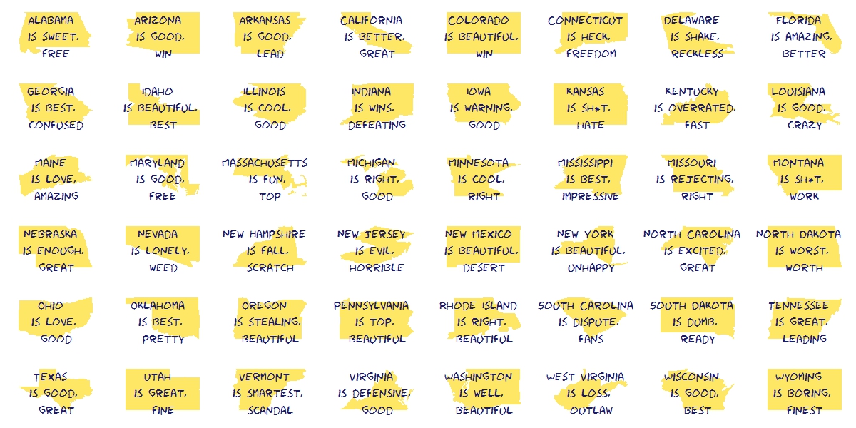
Inspired by the fabulous work of Jonathan Harris I decided to compare human emotions of people living (or twittering in this case) in different cities. My plan was analysing tweets generated in different locations of USA and UK with one thing in common: all of them must contain the string “I FEEL”. These are the main steps I followed:

  • Locate cities I want to analyze using world cities database of maps package
  • Download tweets around these locations using searchTwitter function of twitteR package.
  • Cross tweets with positive and negative lists of words and calculate a simple scoring for each tweet as number of positive words – number of negative words
  • Calculate how many tweets have non-zero scoring; since these tweets put into words some emotion I call them sentimental tweets
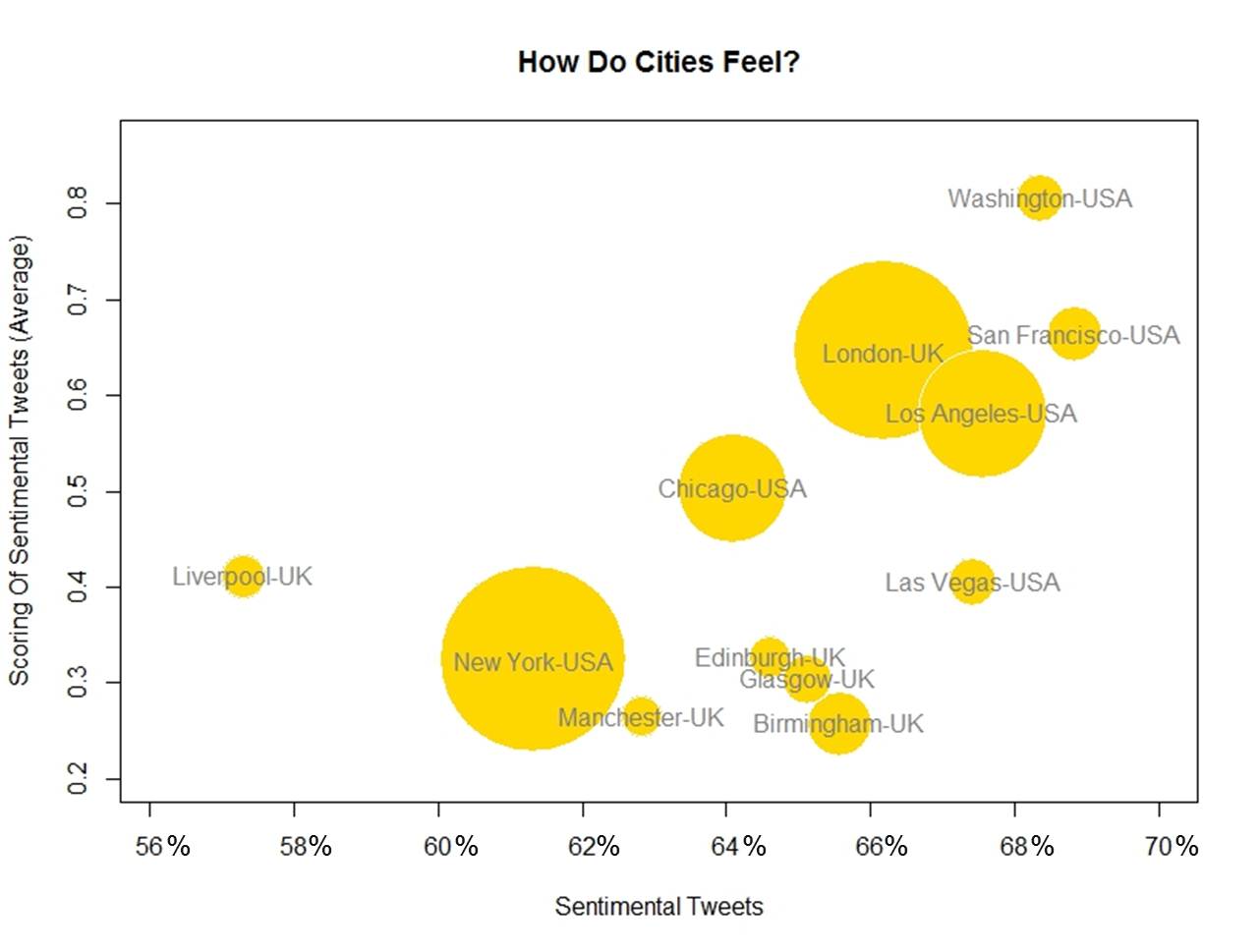
  • Represent cities in a bubble chart where x-axis is percentage of sentimental tweets, y-axis is average scoring and size of bubble is population

This is the result of my experiment:HowDoCitiesFeel3

These are my conclusions (please, do not take it seriously):

  • USA cities seem to have better vibrations and are more sentimental than UK ones
  • Capital city is the happiest one for both countries
  • San Francisco (USA) is the most sentimental city of the analysis; on the other hand, Liverpool (UK) is the coldest one
  • The more sentimental, the better vibrations

From my point of view, this analysis has some important limitations:

  • It strongly depends on particular events (i.e. local football team wins the championship)
  • I have no idea of what kind of people is behind tweets
  • According to my experience, searchTwitter only works well for a small number of searches (no more than 300); for larger number of tweets to return, it use to give malformed JSON response error from server

Anyway, I hope it will serve as starting point of some other analysis in the future. At least, I learned interesting things about R doing it.

Here you have the code:

library(twitteR)
library(RCurl)
library(maps)
library(plyr)
library(stringr)
library(bitops)
library(scales)
#Register
if (!file.exists('cacert.perm'))
{
  download.file(url = 'http://curl.haxx.se/ca/cacert.pem', destfile='cacert.perm')
}
requestURL="https://api.twitter.com/oauth/request_token"
accessURL="https://api.twitter.com/oauth/access_token"
authURL="https://api.twitter.com/oauth/authorize"
consumerKey = "YOUR CONSUMER KEY HERE"
consumerSecret = "YOUR CONSUMER SECRET HERE"
Cred <- OAuthFactory$new(consumerKey=consumerKey,
                         consumerSecret=consumerSecret,
                         requestURL=requestURL,
                         accessURL=accessURL,
                         authURL=authURL)
Cred$handshake(cainfo=system.file("CurlSSL", "cacert.pem", package="RCurl"))
#Save credentials
save(Cred, file="twitter authentification.Rdata")
load("twitter authentification.Rdata")
registerTwitterOAuth(Cred)
options(RCurlOptions = list(cainfo = system.file("CurlSSL", "cacert.pem", package = "RCurl")))
#Cities to analyze
cities=data.frame(
  CITY=c('Edinburgh', 'London', 'Glasgow', 'Birmingham', 'Liverpool', 'Manchester',
         'New York', 'Washington', 'Las Vegas', 'San Francisco', 'Chicago','Los Angeles'),
  COUNTRY=c("UK", "UK", "UK", "UK", "UK", "UK", "USA", "USA", "USA", "USA", "USA", "USA"))
data(world.cities)
cities2=world.cities[which(!is.na(match(
str_trim(paste(world.cities$name, world.cities$country.etc, sep=",")),
str_trim(paste(cities$CITY, cities$COUNTRY, sep=","))
))),]
cities2$SEARCH=paste(cities2$lat, cities2$long, "10mi", sep = ",")
cities2$CITY=cities2$name
#Download tweets
tweets=data.frame()
for (i in 1:nrow(cities2))
{
  tw=searchTwitter("I FEEL", n=400, geocode=cities2[i,]$SEARCH)
  tweets=rbind(merge(cities[i,], twListToDF(tw),all=TRUE), tweets)
}
#Save tweets
write.csv(tweets, file="tweets.csv", row.names=FALSE)
#Import csv file
city.tweets=read.csv("tweets.csv")
#Download lexicon from http://www.cs.uic.edu/~liub/FBS/opinion-lexicon-English.rar
hu.liu.pos = scan('lexicon/positive-words.txt',  what='character', comment.char=';')
hu.liu.neg = scan('lexicon/negative-words.txt',  what='character', comment.char=';')
#Function to clean and score tweets
score.sentiment=function(sentences, pos.words, neg.words, .progress='none')
{
  require(plyr)
  require(stringr)
  scores=laply(sentences, function(sentence, pos.word, neg.words) {
    sentence=gsub('[[:punct:]]','',sentence)
    sentence=gsub('[[:cntrl:]]','',sentence)
    sentence=gsub('\\d+','',sentence)
    sentence=tolower(sentence)
    word.list=str_split(sentence, '\\s+')
    words=unlist(word.list)
    pos.matches=match(words, pos.words)
    neg.matches=match(words, neg.words)
    pos.matches=!is.na(pos.matches)
    neg.matches=!is.na(neg.matches)
    score=sum(pos.matches) - sum(neg.matches)
    return(score)
  }, pos.words, neg.words, .progress=.progress)
  scores.df=data.frame(score=scores, text=sentences)
  return(scores.df)
}
cities.scores=score.sentiment(city.tweets[1:nrow(city.tweets),], hu.liu.pos, hu.liu.neg, .progress='text')
cities.scores$pos2=apply(cities.scores, 1, function(x) regexpr(",",x[2])[1]-1)
cities.scores$CITY=apply(cities.scores, 1, function(x) substr(x[2], 1, x[3]))
cities.scores=merge(x=cities.scores, y=cities, by='CITY')
df1=aggregate(cities.scores["score"], by=cities.scores[c("CITY")], FUN=length)
names(df1)=c("CITY", "TWEETS")
cities.scores2=cities.scores[abs(cities.scores$score)>0,]
df2=aggregate(cities.scores2["score"], by=cities.scores2[c("CITY")], FUN=length)
names(df2)=c("CITY", "TWEETS.SENT")
df3=aggregate(cities.scores2["score"], by=cities.scores2[c("CITY")], FUN=mean)
names(df3)=c("CITY", "TWEETS.SENT.SCORING")
#Data frame with results
df.result=join_all(list(df1,df2,df3,cities2), by = 'CITY', type='full')
#Plot results
radius <- sqrt(df.result$pop/pi)
symbols(100*df.result$TWEETS.SENT/df.result$TWEETS, df.result$TWEETS.SENT.SCORING, circles=radius,
        inches=0.85, fg="white", bg="gold", xlab="Sentimental Tweets", ylab="Scoring Of Sentimental Tweets (Average)",
        main="How Do Cities Feel?")
text(100*df.result$TWEETS.SENT/df.result$TWEETS, df.result$TWEETS.SENT.SCORING, paste(df.result$CITY, df.result$country.etc, sep="-"), cex=1, col="gray50")