Tag Archives: highcharts

Bayesian Blood

The fourth, the fifth, the minor fall and the major lift (Hallelujah, Leonard Cohen)

Next problem is extracted from MacKay’s Information Theory, Inference and Learning Algorithms:

Two people have left traces of their own blood at the scene of a crime. A suspect, Oliver, is tested and found to have type ‘O’ blood. The blood groups of the two traces are found to be of type ‘O’ (a common type in the local population, having frequency 60%) and of type ‘AB’ (a rare type, with frequency 1%). Do these data give evidence in favor of the proposition that Oliver was one of the people who left blood at the scene?

To answer the question, let’s first remember the probability form of Bayes theorem:

p(H|D)=\dfrac{p(H)p(D|H)}{p(D)}

where:

  • p(H) is the probability of the hypothesis H before we see the data, called the prior
  • p(H|D) is the probablity of the hyothesis after we see the data, called the posterior
  • p(D|H) is the probability of the data under the hypothesis, called the likelihood
  • p(D)is the probability of the data under any hypothesis, called the normalizing constant

If we have two hypothesis, A and B, we can write the ratio of posterior probabilities like this:

\dfrac{p(A|D)}{p(B|D)}=\dfrac{p(A)p(D|A)}{p(B)p(D|B)}

If p(A)=1-p(B) (what means that A and B are mutually exclusive and collective exhaustive), then we can rewrite the ratio of the priors and the ratio of the posteriors as odds. Writing o(A) for odds in favor of A, we get the odds form of Bayes theorem:

o(A|D)=o(A)\dfrac{p(D|A)}{p(D|B)}

Dividing through by o(A) we have:

\dfrac{o(A|D)}{o(A)}=\dfrac{p(D|A)}{p(D|B)}

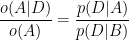
The term on the left is the ratio of the posteriors and prior odds. The term on the right is the likelihood ratio, also called the Bayes factor. If it is greater than 1, that means that the data were more likely under A than under B. And since the odds ratio is also greater than 1, that means that the odds are greater, in light of the data, than they were before. If the Bayes factor is less than 1, that means the data were less likely under A than under B, so th odds in favor of A go down.

Let’s go back to our initial problem. If Oliver left his blood at the crime scene, the probability of the data is just the probability that a random member of the population has type ‘AB’ blood, which is 1%. If Oliver did not leave blood at the scene, what is the the chance of finding two people, one with type ‘O’ and one with type ‘AB’? There are two ways it might happen: the first person we choose might have type ‘O’ and the second ‘AB’, or the other way around. So the probability in this case is 2(0.6)(0.01)=1.2%. Dividing probabilities of both scenarios we obtain a Bayes factor of 0.83, and we conclude that the blood data is evidence against Oliver’s guilt.

Once I read this example, I decided to replicate it using real data of blood type distribution by country from here. After cleaning data, I have this nice data set to work with:

For each country, I get the most common blood type (the one which the suspect has) and the least common and replicate the previous calculations. For example, in the case of Spain, the most common type is ‘O+’ with 36% and the least one is ‘AB-‘ with 0.5%. The Bayes factor is 0.005/(2(0.36)(0.005))=1.39 so data support the hypothesis of guilt in this case. Next chart shows Bayes factor accross countries:

Just some comments:

  • Sometimes data consistent with a hypothesis are not necessarily in favor of the hypothesis
  • How different is the distribution of blood types between countries!
  • If you are a estonian ‘A+’ murderer, choose carefully your accomplice

This is the code of the experiment:

library(rvest)
library(dplyr)
library(stringr)
library(DT)
library(highcharter)

# Webscapring of the table with the distribution of blood types
url <- "http://www.rhesusnegative.net/themission/bloodtypefrequencies/"
blood <- url %>%
   read_html() %>%
   html_node(xpath='/html/body/center/table') %>%
   html_table(fill=TRUE)

# Some data cleansing
blood %>% slice(-c(66:68)) -> blood

blood[,-c(1:2)] %>% 
  sapply(gsub, pattern=",", replacement=".") %>% 
  as.data.frame %>% 
  sapply(gsub, pattern=".79.2", replacement=".79") %>% 
  as.data.frame-> blood[,-c(1:2)]

blood %>% 
  sapply(gsub, pattern="%|,", replacement="") %>% 
  as.data.frame -> blood

blood[,-1] = apply(blood[,-1], 2, function(x) as.numeric(as.character(x)))


blood[,-c(1:2)] %>% mutate_all(funs( . / 100)) -> blood[,-c(1:2)]

# And finally, we have a nice data set
datatable(blood, 
          rownames = FALSE,
          options = list(
          searching = FALSE,
          pageLength = 10)) %>% 
  formatPercentage(3:10, 2)

# Calculate the Bayes factor
blood %>% 
  mutate(factor=apply(blood[,-c(1,2)], 1, function(x) {min(x)/(2*min(x)*max(x))})) %>% 
  arrange(factor)-> blood

# Data Visualization
highchart() %>% 
     hc_chart(type = "column") %>% 
     hc_title(text = "Bayesian Blood") %>%
     hc_subtitle(text = "An experiment about the Bayes Factor") %>%  
     hc_xAxis(categories = blood$Country, 
             labels = list(rotation=-90, style = list(fontSize = "12px")))  %>% 
     hc_yAxis(plotBands = list(list(from = 0, to = 1, color = "rgba(255,215,0, 0.8)"))) %>% 
     hc_add_series(data = blood$factor,
                   color = "rgba(255, 0, 0, 0.5)",
                   name = "Bayes Factor")%>% 
  hc_yAxis(min=0.5) %>% 
  hc_tooltip(pointFormat = "{point.y:.2f}") %>% 
  hc_legend(enabled = FALSE) %>% 
  hc_exporting(enabled = TRUE) %>%
  hc_chart(zoomType = "xy")

Visualizing the Daily Variability of Bitcoin with Quandl and Highcharts

Lay your dreams, little darling, in a flower bed; let that sunshine in your hair (Where the skies are blue, The Lumineers)

I discovered this nice visualization some days ago. The author is also the creator of Highcharter, an incredible R wrapper for Highcharts javascript libray and its modules. I am a big fan of him.

Inspired by his radial plot, I did a visualization of the daily evolution of Daily Bitcoin exchange rate (BTC vs. EUR) on Localbtc. Data is sourced from here and I used Quandl to obtain the data frame. Quandl is a marketplace for financial and economic data delivered in modern formats for today’s analysts. There is a package called Quandl to interact directly with the Quandl API to download data in a number of formats usable in R. You only need to locate the data you want in the Quandl site. In my case data are here.

After loading data, I do the folowing steps:

  • Filtering data to obtain last 12 complete months
  • Create a new variable with the difference between closing and opening price of Bitcoin (in Euros)
  • Create a color variable to distinguish between positive and negative differences
  • Create the graph using Fivethirtyeight theme for highcharts

This is the result:

Apart of its appealing, I think is a good way to to have a quick overview of the evolution of a stock price. This is the code to do the experiment:

library(Quandl)
library(dplyr)
library(highcharter)
library(lubridate)
bitcoin=Quandl("BCHARTS/LOCALBTCEUR")
bitcoin %>% 
  arrange(Date) %>% 
  mutate(tmstmp = datetime_to_timestamp(Date)) -> bitcoin
last_date=max(bitcoin$Date)
if (day(last_date+1)==1) date_to=last_date else 
  date_to=ymd(paste(year(last_date), month(last_date),1, sep="-"))-1
date_from=ymd(paste(year(date_to)-1, month(date_to)+1,1, sep="-"))
bitcoin %>% filter(Date>=date_from, Date<=date_to) -> bitcoin
var_bitcoin <- bitcoin %>% 
  mutate(Variation = Close - Open,
         color = ifelse(Variation>=0, "green", "red"),
         y = Variation) %>% 
  select(x = tmstmp,
         y,
         variation = Variation,
         name = Date,
         color,
         open = Open,
         close = Close) %>% 
  list.parse3()
x <- c("Open", "Close", "Variation")
y <- sprintf("{point.%s}", tolower(x))
tltip <- tooltip_table(x, y)
hc <- highchart() %>% 
  hc_title(text = "Bitcoin Exchange Rate (BTC vs. EUR)") %>% 
  hc_subtitle(text = "Daily Variation on Localbtc. Last 12 months")%>% 
  hc_chart(
    type = "column",
    polar = TRUE) %>%
  hc_plotOptions(
    series = list(
      stacking = "normal",
      showInLegend = FALSE)) %>% 
  hc_xAxis(
    gridLineWidth = 0.5,
    type = "datetime",
    tickInterval = 30 * 24 * 3600 * 1000,
    labels = list(format = "{value: %b}")) %>% 
  hc_yAxis(showFirstLabel = FALSE) %>% 
  hc_add_series(data = var_bitcoin) %>% 
  hc_add_theme(hc_theme_538()) %>% 
  hc_tooltip(useHTML = TRUE,
    headerFormat = as.character(tags$small("{point.x:%d %B, %Y}")),
    pointFormat = tltip)
hc

Visualizing the Gender of US Senators With R and Highmaps

I wake up every morning in a house that was built by slaves (Michelle Obama)

Some days ago I was invited by the people of Highcharts to write a post in their blog. What I have done is a simple but revealing map of women senators of the United States of America. Briefly, this is what I’ve done to generate it:

  • read from the US senate website a XML file with senators info
  • clean and obtain gender of senators from their first names
  • summarize results by state
  • join data with a US geojson dataset to create the highmap

You can find details and R code here.

It is easy creating a highcharts using highcharter, an amazing library as genderizeR, the one I use to obtain gender names. I like them a lot.

The Hype Bubble Map for Dog Breeds

In the whole history of the world there is but one thing that money can not buy… to wit the wag of a dog’s tail (Josh Billings)

In this post I combine several things:

  • Simple webscraping to read the list of companion dogs from Wikipedia. I love rvest package to do these things
  • Google Trends queries to download the evolution of searchings of breeds during last 6 months. I use gtrendsR package to do this and works quite well
  • A dinamic Highchart visualization using the awesome highcharter package

The experiment is based on a simple idea: what people search on the Internet is what people do. Can be Google Trends an useful tool to know which breed will become fashionable in the future? To be honest, I don’t really know but I will make my own bet.

What I have done is to extract last 6 months of Google trends of this list of companion breeds. After some simple text mining, I divide the set of names into 5-elements subsets because Google API doesn’t allow searchings with more than 5 items. The result of the query to Google trends is a normalized time series, meaning the 0 – 100 values are relative, not absolute, measures. This is done by taking all of the interest data for your keywords and dividing it by the highest point of interest for that date range. To make all 5-items of results comparable I always include King Charles Spaniel breed in all searchings (as a kind of undercover agent I will use to compare searching levels). The resulting number is my “Level” Y-Axis of the plot. I limit searchings to code=”0-66″ which is restrict results to Animals and pets category. Thanks, Philippe, for your help in this point. I also restrict rearchings To the United States of America.

There are several ways to obtain an aggregated trend indicator of a time series. My choice here was doing a short moving average order=2 to the resulting interest over time obtained from Google. The I divide the weekly variations by the smoothed time series. The trend indicator is the mean of these values. To obtains a robust indicator, I remove outliers of the original time series. This is my X-axis.

I discovered recently a wonderful package called highcharter which allows you to create incredibly cool dynamic visualizations. I love it and I could not resist to use it to do the previous plot with the look and feel of The Economist:

Inspired by Gartner’s Hype Cycle of Emerging Technologies I distinguish two sets of dog breeds:

  • Plateau of Productivity Breeds (succesful breeds with very high level indicator and possitive trend): Golden Retriever, Pomeranian, Chihuahua, Collie and Shih Tzu.
  • Innovation Trigger Breeds (promising dog breeds with very high trend indicator and low level): Mexican Hairless Dog, Keeshond, West Highland White Terrier and German Spitz.

And here comes my prediction. After analyzing the set Innovation Trigger Breeds, my bet is Keeshond will increase its popularity in the nearly future: don’t you think it is lovely?

640px-Little_Puppy_Keeshond
Photo by Terri BrownFlickr: IMG_4723, CC BY 2.0

Here you have the code:

library(gtrendsR)
library(rvest)
library(dplyr)
library(stringr)
library(forecast)
library(outliers)
library(highcharter)
library(ggplot2)
library(scales)
 
x="https://en.wikipedia.org/wiki/Companion_dog"
read_html(x) %>% 
  html_nodes("ul:nth-child(19)") %>% 
  html_text() %>% 
  strsplit(., "\n") %>% 
  unlist() -> breeds
breeds=iconv(breeds[breeds!= ""], "UTF-8")
usr <- "YOUR GOOGLE ACCOUNT"
psw <- "YOUR GOOGLE PASSWORD"
gconnect(usr, psw)
#Reference
ref="King Charles Spaniel"
#New set
breeds=setdiff(breeds, ref)
#Subsets. Do not worry about warning message
sub.breeds=split(breeds, 1:ceiling(length(breeds)/4))
results=list()
for (i in 1:length(sub.breeds))
{
  res <- gtrends(unlist(union(ref, sub.breeds[i])), 
          start_date = Sys.Date()-180,
          cat="0-66",
          geo="US")
  results[[i]]=res
}
trends=data.frame(name=character(0), level=numeric(0), trend=numeric(0))
for (i in 1:length(results))
{
  df=results[[i]]$trend
  lr=mean(results[[i]]$trend[,3]/results[[1]]$trend[,3])
  for (j in 3:ncol(df))
  {
    s=rm.outlier(df[,j], fill = TRUE)
    t=mean(diff(ma(s, order=2))/ma(s, order=2), na.rm = T)
    l=mean(results[[i]]$trend[,j]/lr)
    trends=rbind(data.frame(name=colnames(df)[j], level=l, trend=t), trends)
  }
}
 
trends %>% 
  group_by(name) %>% 
  summarize(level=mean(level), trend=mean(trend*100)) %>% 
  filter(level>0 & trend > -10 & level<500) %>% 
  na.omit() %>% 
  mutate(name=str_replace_all(name, ".US","")) %>% 
  mutate(name=str_replace_all(name ,"[[:punct:]]"," ")) %>% 
  rename(
    x = trend,
    y = level
  ) -> trends
trends$y=(trends$y/max(trends$y))*100
#Dinamic chart as The Economist
highchart() %>% 
  hc_title(text = "The Hype Bubble Map for Dog Breeds") %>%
  hc_subtitle(text = "According Last 6 Months of Google Searchings") %>% 
  hc_xAxis(title = list(text = "Trend"), labels = list(format = "{value}%")) %>% 
  hc_yAxis(title = list(text = "Level")) %>% 
  hc_add_theme(hc_theme_economist()) %>%
  hc_add_series(data = list.parse3(trends), type = "bubble", showInLegend=FALSE, maxSize=40) %>% 
  hc_tooltip(formatter = JS("function(){
                            return ('<b>Trend: </b>' + Highcharts.numberFormat(this.x, 2)+'%' + '<br><b>Level: </b>' + Highcharts.numberFormat(this.y, 2) + '<br><b>Breed: </b>' + this.point.name)
                            }"))