The fourth, the fifth, the minor fall and the major lift (Hallelujah, Leonard Cohen)
Next problem is extracted from MacKay’s Information Theory, Inference and Learning Algorithms:
Two people have left traces of their own blood at the scene of a crime. A suspect, Oliver, is tested and found to have type ‘O’ blood. The blood groups of the two traces are found to be of type ‘O’ (a common type in the local population, having frequency 60%) and of type ‘AB’ (a rare type, with frequency 1%). Do these data give evidence in favor of the proposition that Oliver was one of the people who left blood at the scene?
To answer the question, let’s first remember the probability form of Bayes theorem:

where:
- p(H) is the probability of the hypothesis H before we see the data, called the prior
- p(H|D) is the probablity of the hyothesis after we see the data, called the posterior
- p(D|H) is the probability of the data under the hypothesis, called the likelihood
- p(D)is the probability of the data under any hypothesis, called the normalizing constant
If we have two hypothesis, A and B, we can write the ratio of posterior probabilities like this:

If p(A)=1-p(B) (what means that A and B are mutually exclusive and collective exhaustive), then we can rewrite the ratio of the priors and the ratio of the posteriors as odds. Writing o(A) for odds in favor of A, we get the odds form of Bayes theorem:

Dividing through by o(A) we have:
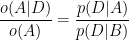
The term on the left is the ratio of the posteriors and prior odds. The term on the right is the likelihood ratio, also called the Bayes factor. If it is greater than 1, that means that the data were more likely under A than under B. And since the odds ratio is also greater than 1, that means that the odds are greater, in light of the data, than they were before. If the Bayes factor is less than 1, that means the data were less likely under A than under B, so th odds in favor of A go down.
Let’s go back to our initial problem. If Oliver left his blood at the crime scene, the probability of the data is just the probability that a random member of the population has type ‘AB’ blood, which is 1%. If Oliver did not leave blood at the scene, what is the the chance of finding two people, one with type ‘O’ and one with type ‘AB’? There are two ways it might happen: the first person we choose might have type ‘O’ and the second ‘AB’, or the other way around. So the probability in this case is 2(0.6)(0.01)=1.2%. Dividing probabilities of both scenarios we obtain a Bayes factor of 0.83, and we conclude that the blood data is evidence against Oliver’s guilt.
Once I read this example, I decided to replicate it using real data of blood type distribution by country from here. After cleaning data, I have this nice data set to work with:
For each country, I get the most common blood type (the one which the suspect has) and the least common and replicate the previous calculations. For example, in the case of Spain, the most common type is ‘O+’ with 36% and the least one is ‘AB-‘ with 0.5%. The Bayes factor is 0.005/(2(0.36)(0.005))=1.39 so data support the hypothesis of guilt in this case. Next chart shows Bayes factor accross countries:
Just some comments:
- Sometimes data consistent with a hypothesis are not necessarily in favor of the hypothesis
- How different is the distribution of blood types between countries!
- If you are a estonian ‘A+’ murderer, choose carefully your accomplice
This is the code of the experiment:
library(rvest)
library(dplyr)
library(stringr)
library(DT)
library(highcharter)

# Webscapring of the table with the distribution of blood types
url <- "http://www.rhesusnegative.net/themission/bloodtypefrequencies/"
blood <- url %>%
   read_html() %>%
   html_node(xpath='/html/body/center/table') %>%
   html_table(fill=TRUE)

# Some data cleansing
blood %>% slice(-c(66:68)) -> blood

blood[,-c(1:2)] %>%
  sapply(gsub, pattern=",", replacement=".") %>%
  as.data.frame %>%
  sapply(gsub, pattern=".79.2", replacement=".79") %>%
  as.data.frame-> blood[,-c(1:2)]

blood %>%
  sapply(gsub, pattern="%|,", replacement="") %>%
  as.data.frame -> blood

blood[,-1] = apply(blood[,-1], 2, function(x) as.numeric(as.character(x)))


blood[,-c(1:2)] %>% mutate_all(funs( . / 100)) -> blood[,-c(1:2)]

# And finally, we have a nice data set
datatable(blood,
          rownames = FALSE,
          options = list(
          searching = FALSE,
          pageLength = 10)) %>%
  formatPercentage(3:10, 2)

# Calculate the Bayes factor
blood %>%
  mutate(factor=apply(blood[,-c(1,2)], 1, function(x) {min(x)/(2*min(x)*max(x))})) %>%
  arrange(factor)-> blood

# Data Visualization
highchart() %>%
     hc_chart(type = "column") %>%
     hc_title(text = "Bayesian Blood") %>%
     hc_subtitle(text = "An experiment about the Bayes Factor") %>%
     hc_xAxis(categories = blood$Country,
             labels = list(rotation=-90, style = list(fontSize = "12px")))  %>%
     hc_yAxis(plotBands = list(list(from = 0, to = 1, color = "rgba(255,215,0, 0.8)"))) %>%
     hc_add_series(data = blood$factor,
                   color = "rgba(255, 0, 0, 0.5)",
                   name = "Bayes Factor")%>%
  hc_yAxis(min=0.5) %>%
  hc_tooltip(pointFormat = "{point.y:.2f}") %>%
  hc_legend(enabled = FALSE) %>%
  hc_exporting(enabled = TRUE) %>%
  hc_chart(zoomType = "xy")
I was delighted by the explanation of the Bayes factor. Owing to you mentioning it, I finally grabbed a copy of the late Sir David MacKay’s book from the library. It is a true wonder.
Side question: did you exclude the United States and the United Kingdom on purpose?
Thanks! I don’t know why I lost them. I will check it out and will modify my code to recover them.
Fixed! Thanks!
Isn’t
min(x)/(2*min(x)*max(x))
just the same thing as
1/(2*max(x))
unless min(x) = 0 when the ratio is undefined? What role does min(x) play in the Bayes factor here, in other word?
min(x) is the % of least common blood and max(x) is the % of most common blood. The formula is the application of bayes factor for these blood types.
Where you say “If p(B)=1-p(B) (what means that A and B are mutually exclusive and collective exhaustive)” do you mean “p(B)=1-p(A)” ?
Yes. Thanks
fixed!
Well that was really thought provoking, but not quite in the way intended.
I am disturbed by this counter-intuitive result. If there were just one blood stain of type O then the Bayes factor would be about 1.7. Finding another blood stain of a different type halved the factor – that feels really odd. In both cases the factor depends only on the prevalence of type O blood and not of the other type.
Suppose it were not the familiar blood types, but some other variant that was tested and that Oliver’s measurement that matched one stain was shared with 99.9% of the population, then the Bayes factor would be little more than one half. Do you have an explanation to make this more common-sensible?
I wonder whether the problem lies in the o(A) – the a priori odds of Oliver’s being guilty – i.e. before any blood type data is taken into account. I’m not that happy with it, but my favourite approach so far is to consider the probabilities conditional on the number of perpetrators. The more perpetrators there are, the higher the a priori likelihood that Oliver is one of them. My suspicion is that this effect pretty much cancels out the reduction in the Bayes factor that apparently results from the discovery that one of the blood stains cannot be Oliver’s.
Hi,
Why are we multiplying (0.6)(0.01) by 2? Why do we care about the order in this case? How does it matter if the first person had O and another had AB and the other way round?
That’s because both events are taken as being independent so there are two possible cases. It doesn’t matter the order. Think about picking people from a bag: there are two options: the first one you pick is O and the other is AB or the opposite.
Coming back to this after such a long gap I think I see what is going on – and it is pretty much as I suspected.
If there are N possible suspects and no reason to suspect Oliver then you might assume that the a priori probability of Oliver being guilty is 1/N. But as there are two perpetrators then the a priori probability that one of them is Oliver doubles to 2/N. The a posteriori probability that Oliver was there is increased by the finding of blood matching his group and reduced by the finding of a trace that doesn’t match. It turns out that if the prevalence of Oliver’s blood group is more than 50% then the reduction is more than the increase and that surprises us for some reason.