The heart has its reasons which reason knows not (Blaise Pascal)
You only need two functions to draw a heart mathematically. The upper part is generated by (1-(|x|-1)2)1/2 and the lower one by acos(1-|x|)-PI. Here is how this heart is:

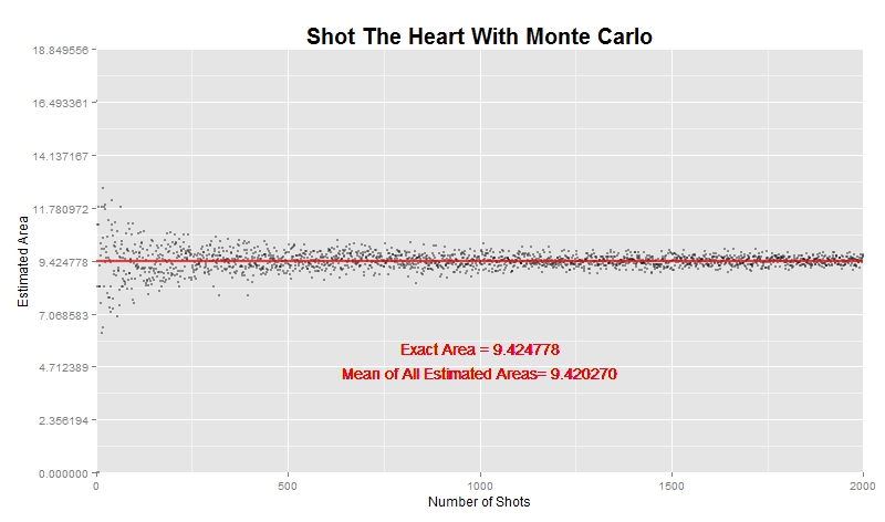
Whats the area of this heart? It’s easy: integrating heart.up(x)-heart.dw(x) between -2 and 2 and you will obtain that heart measures 9.424778, but there is a simple and nice way to approximate to this value: shoot the heart.
The idea is very simple. Heart is delimited by a square with vertex in (-2, heart.dw(0)), (-2, 1), (2, heart.dw(0)) and (2, 1). Generating a set of points uniformly distributed inside the square and counting how many of them fall into the heart in relation to the area of the square gives a very good approximation of the exact area of the heart. This is a plot representing a simulation of 2.000 shots (hits in red, fails in blue):

Given a simulation of n points, the estimated area of the heart is the area of the square by percentage of points that falls inside the heart. And of course, precision increases with the number of shots you make, as you can see in the following plot, where exact area is represented by the red horizontal line:
Here you have the code:
library("ggplot2")
heart.up <- function(x) {sqrt(1-(abs(x)-1)^2)} #Upper part of the heart
heart.dw <- function(x) {acos(1-abs(x))-pi}    #Lower part of the heart
#Plot of the heart
ggplot(data.frame(x=c(-2,2)), aes(x)) +
  stat_function(fun=heart.up, geom="line", aes(colour="heart.up")) +
  stat_function(fun=heart.dw, geom="line", aes(colour="heart.dw")) +
  scale_colour_manual("Function", values=c("blue","red"), breaks=c("heart.up","heart.dw"))+
  labs(x = "", y = "")+
  theme(legend.position = c(.85, .15))
sims <- 2000 #Number of simulations
rlts <- data.frame()
for (i in 1:sims)
  {
  msm <- cbind(as.matrix(runif(i, min=-2, max=2)), as.matrix(runif(i, min=heart.dw(0), max=1)))
  nin <- 0
  for (j in 1:nrow(msm)) {if (msm[j,2]<=heart.up(msm[j,1]) & msm[j,2]>=heart.dw(msm[j,1])) nin=nin+1}
  rlts <- rbind(c(i, 4*(1-heart.dw(0))*nin/i), rlts)
  }
colnames(rlts) <- c("no.simulations","heart.area")
exact.area <- integrate(function(x) {heart.up(x)-heart.dw(x)},-2,2)$value
mean.area <- mean(rlts$heart.area) #Mean of All Estimated Areas
ggplot(data = rlts, aes(x = no.simulations, y = heart.area))+
  geom_point(size = 0.5, colour = "black", alpha=0.4)+
  geom_abline(intercept = exact.area, slope = 0, size = 1, linetype=1, colour = "red", aes(color="My Line"), alpha=0.8, show_guide = TRUE)+
  labs(list(x = "Number of Shots", y = "Estimated Area"))+
  ggtitle("Shot The Heart With Monte Carlo") +
  theme(plot.title = element_text(size=20, face="bold"))+
  scale_x_continuous(limits = c(0, sims), expand = c(0, 0))+
  expand_limits(x = 0, y = 0)+
  scale_y_continuous(limits = c(0, 2*exact.area), expand = c(0, 0), breaks=c(0, exact.area/4, exact.area/2, 3*exact.area/4, exact.area, 5*exact.area/4, 3*exact.area/2, 7*exact.area/4, 2*exact.area))+
  geom_text(x = 1000, y = exact.area/2, label=paste("Exact Area =", sprintf("%7.6f", exact.area)), vjust=-1, colour="red", size=5)+
  geom_text(x = 1000, y = exact.area/2, label=paste("Mean of All Estimated Areas=", sprintf("%7.6f", mean.area)), vjust=+1, colour="red", size=5)