Tag Archives: Madrid

The Cycling Accident Map of Madrid City

Far away, this ship has taken me far away (Starlight, Muse)

Madrid City has an Open Data platform where can be found around 300 data sets about a number of topics. One of these sets is the one I used for this experiment. It contains information about cycling accidents  happened in the city from January to July 2017. I have done a map to locate where the accidents took place. This experiment shows how R makes very easy to create professional maps with Leaflet (in this case I use Carto basemaps).

To locate accidents the data set only contains the address where they happened so the first thing I did is to obtain their geographical coordinates using geocode function from ggmap package. There were 431 accidents during the first 7 months of 2017 (such a big number!) and I got coordinates of 407 so I can locate 94% of the accidents.

Obviously, the amount of accidents in some place depend on how many bikers circulate there as well as on its infrastructure. None of these things can be seen in the map: It only shows number of accidents.

The categorization of accidents is:

  • Double collision (Colisión doble): Traffic accident occurred between two moving vehicles.
  • Multiple collision (Colisión múltiple): Traffic accident occurred between more than two moving vehicles.
  • Fixed object collision (Choque con objeto fijo): Accident occurred between a moving vehicle with a driver and an immovable object that occupies the road or separated area of ​​the same, whether parked vehicle, tree, street lamp, etc.
  • Accident (Atropello): Accident occurred between a vehicle and a pedestrian that occupies the road or travels by sidewalks, refuges, walks or zones of the public road not destined to the circulation of vehicles.
  • Overturn (Vuelco): Accident suffered by a vehicle with more than two wheels which by some circumstance loses contact with the road and ends supported on one side or on its roof.
  • Motorcycle fall (Caída motocicleta): Accident suffered by a motorcycle, which at some moment loses balance, because of the driver or due to the conditions of the road.
  • Moped fall (Caída ciclomotor): Accident suffered by a moped, which at some moment loses balance, because of the driver or due to the conditions of the road.
  • Bicycle fall (Caída bicicleta): Accident suffered by a bicycle, which at some moment loses balance, because of the driver or due to the conditions of the road.

These categories are redundant (e.g. Double and Multiple collision), difficult to understand (e.g. Overturn) or both things at the same time (e.g. Motorcycle fall and Moped fall). This categorization also forgets human damages incurred by the accident.

Taking all these things in mind, this is the map:

Here is a full-screen version of the map.

My suggestions to the city council of Madrid are:

  1. Add geographical coordinates to data (I guess many of the analysis will need them)
  2. Rethink the categorization to make it clearer and more informative
  3. Add more cycling data sets to the platform (detail of bikeways, traffic …) to understand accidents better
  4. Attending just to the number of accidents , put the focus around Parque del Retiro, specially on its west surroundings, from Plaza de Cibeles to Plaza de Carlos V: more warning signals, more  (or better) bikeways …

I add the code below to update the map (If someone ask it to me, I can do it myself regularly):

library(dplyr)
library(stringr)
library(ggmap)
library(leaflet)
# First, getting the data
download.file(paste0("http://datos.madrid.es/egob/catalogo/", file), 
              destfile="300110-0-accidentes-bicicleta.csv")

data=read.csv("300110-0-accidentes-bicicleta.csv", sep=";", skip=1)

# Prepare data for geolocation
data %>% 
  mutate(direccion=paste(str_trim(Lugar), str_trim(Numero), "MADRID, SPAIN", sep=", ") %>% 
           str_replace("NA, ", "") %>% 
           str_replace(" - ", " CON ")) -> data

# Geolocation (takes some time ...)
coords=c()
for (i in 1:nrow(data)) 
{
  coords %>% rbind(geocode(data[i,"direccion"])) -> coords
  Sys.sleep(0.5)
}
  
# Save data, just in case
data %>% cbind(coords) %>% saveRDS(file="bicicletas.RDS")

data=readRDS(file="bicicletas.RDS")

# Remove non-successfull geolocations
data %>% 
  filter(!is.na(lon)) %>% 
  droplevels()-> data

# Remove non-successfull geolocations
data %>% mutate(Fecha=paste0(as.Date(data$Fecha, "%d/%m/%Y"), " ", TRAMO.HORARIO),
                popup=paste0("<b>Dónde:</b>",
                             direccion,
                             "<b>Cuándo:</b>",
                             Fecha,
                             "<b>Qué pasó:</b>",
                             Tipo.Accidente)) -> data

# Do the map
data %>% split(data$Tipo.Accidente) -> data.df

l <- leaflet() %>% addProviderTiles(providers$CartoDB.Positron)

names(data.df) %>%
  purrr::walk( function(df) {
    l <<- l %>%
      addCircleMarkers(data=data.df[[df]],
                 lng=~lon, lat=~lat,
                 popup=~popup,
                 color="red",
                 stroke=FALSE,
                 fillOpacity = 0.8,
                 group = df,
                 clusterOptions = markerClusterOptions(removeOutsideVisibleBounds = F))
  })

l %>%
  addLayersControl(
    overlayGroups = names(data.df),
    options = layersControlOptions(collapsed = FALSE)
  )
Analysing The Rock ‘n’ Roll Madrid Marathon

Nobody’s going to win all the time. On the highway of life you can’t always be in the fast lane (Haruki Murakami, What I Talk About When I Talk About Running)

I started running two years ago and one if my dreams is to run a marathon someday. One month ago I run my first half marathon so this day is become closer but I am in no hurry to do it. Meanwhile, I prefer analysing the results of the last edition of the Rock ‘n’ Roll Madrid marathon which, by the way, will be hold again next weekend. This is the first time I do webscraping to download data from a website and it has been quite easy thanks to rvest package.

Once I go over this website form, I have timings of every runner (more than 11.000) at 5, 10, 15, 20, 21.097, 25, 30, 35, 40, and 42.195 kilometers. This, togheter with the category of each runner is the base for my analysis. I remove categories with a small number of runners.

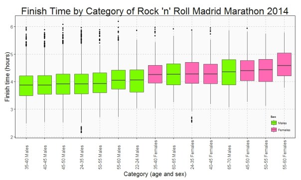
This is the Box plot of the finish time by category:

Finish Time

Who maintains the rhythm better? Since I have the time at the end and at the middle (21.097 km), I can do a Box plot with the variation time between first and second half of the Marathon:

Variation Time

Only a handful of people pull out of the Marathon before finishing but once again this rate is not the same between categories. This is the survival rate by category along the race:

Survival Rate

This plots show some interesting things:

  • Fastest category is 35-40 years old for both genders
  • Fastest individuals are inside 24-35 years old for both genders
  • Youngest ages are not the fastest
  • Between 40-45 category is the second fastest for men and the third one for women
  • Females between 40-45 keep the most constant rhythm of all categories.
  • Young men between 22-24 years old are the most unconstant: their second half rhythm is much slower than the first one.
  • All females between 55-60 years old ended the marathon
  • On the other hand, males between 60-65 are the category with most ‘deads’ during the race

Long life forties:

library(rvest)
library(lubridate)
library(ggplot2)
library(plyr)
library(sqldf)
library(scales)
library(gplots)
setwd("YOUR WORKING DIRECTORY HERE")
maraton_web="http://www.maratonmadrid.org/resultados/clasificacion.asp?carrera=13&parcial=par1&clasificacion=1&dorsal=&nombre=&apellidos=&pais=&pagina=par2"
#Grid with parameters to navigate in the web to do webscraping
searchdf=rbind(expand.grid( 1, 0:32), expand.grid( 2, 0:55), expand.grid( 3, 0:56), expand.grid( 4, 0:56),
               expand.grid( 5, 0:56), expand.grid( 6, 0:55), expand.grid( 7, 0:55), expand.grid( 8, 0:55),
               expand.grid( 9, 0:53), expand.grid(10, 0:55))
colnames(searchdf)=c("parcial", "pagina")
#Webscraping. I open the webpage and download the related table with partial results
results=data.frame()
for (i in 1:nrow(searchdf))
{
  maraton_tmp=gsub("par2", searchdf[i,2], gsub("par1", searchdf[i,1], maraton_web))
  df_tmp=html(maraton_tmp) %>% html_nodes("table") %>% .[[3]] %>% html_table()
  results=rbind(results, data.frame(searchdf[i,1], df_tmp[,1:7]))
}
#Name the columns
colnames(results)=c("Partial", "Place", "Bib", "Name", "Surname", "Cat", "Gross", "Net")
#Since downloadind data takes time, I save results in RData format
save(results, file="results.RData")
load("results.RData")
#Translate Net timestamp variable into hours
results$NetH=as.numeric(dhours(hour(hms(results$Net)))+dminutes(minute(hms(results$Net)))+dseconds(second(hms(results$Net))))/3600
results$Sex=substr(results$Cat, 3, 4)
#Translate Cat into years and gender
results$Cat2=revalue(results$Cat, 
                     c("A-F"="18-22 Females", "A-M"="18-22 Males", "B-F"="22-24 Females", "B-M"="22-24 Males", "C-F"="24-35 Females", "C-M"="24-35 Males", 
                       "D-F"="35-40 Females", "D-M"="35-40 Males", "E-F"="40-45 Females", "E-M"="40-45 Males", "F-F"="45-50 Females", "F-M"="45-50 Males", 
                       "G-F"="50-55 Females", "G-M"="50-55 Males", "H-F"="55-60 Females", "H-M"="55-60 Males", "I-F"="60-65 Females", "I-M"="60-65 Males", 
                       "J-F"="65-70 Females", "J-M"="65-70 Males", "K-F"="+70 Females", "K-M"="+70 Males"))
#Translate partial code into kilometers
results$PartialKm=mapvalues(results$Partial, from = c(1, 2, 3, 4, 5, 6, 7, 8, 9, 10), to = c(5, 10, 15, 20, 21.097, 25, 30, 35, 40, 42.195))
#There are some categories with very few participants. I will remove from the analysis
count(subset(results, Partial==10), "Cat")
#General options for ggplot
opts=theme(
  panel.background = element_rect(fill="gray98"),
  panel.border = element_rect(colour="black", fill=NA),
  axis.line = element_line(size = 0.5, colour = "black"),
  axis.ticks = element_line(colour="black"),
  panel.grid.major = element_line(colour="gray75", linetype = 2),
  panel.grid.minor = element_blank(),
  axis.text = element_text(colour="gray25", size=15),
  axis.title = element_text(size=20, colour="gray10"),
  legend.key = element_blank(),
  legend.background = element_blank(),
  plot.title = element_text(size = 32, colour="gray10"))
#Data set with finish times
results1=subset(results, Partial==10 & !(Cat %in% c("A-F", "A-M", "B-F", "I-F", "J-F", "K-F", "K-M")))
ggplot(results1, aes(x=reorder(Cat2, NetH, FUN=median), y=NetH)) + geom_boxplot(aes(fill=Sex), colour = "gray25")+
  scale_fill_manual(values=c("hotpink", "lawngreen"), name="Sex", breaks=c("M", "F"), labels=c("Males", "Females"))+
  labs(title="Finish Time by Category of Rock 'n' Roll Madrid Marathon 2014", x="Category (age and sex)", y="Finish time (hours)")+
  theme(axis.text.x = element_text(angle = 90, vjust=.5, hjust = 0), legend.justification=c(1,0), legend.position=c(1,0))+opts
#Data set with variation times
results2=sqldf("SELECT 
               a.Bib, a.Sex, b.Cat2, (a.NetH-2*b.NetH)*60 as VarMin
               FROM results1 a INNER JOIN results b ON (a.Bib = b.Bib AND b.Partial=5) order by VarMin asc")
ggplot(results2, aes(x=reorder(Cat2, VarMin, FUN=median), y=VarMin)) + geom_boxplot(aes(fill=Sex))+
  scale_fill_manual(values=c("hotpink", "lawngreen"), name="Sex", breaks=c("M", "F"), labels=c("Males", "Females"))+
  labs(title="Time Variation by Category Between First and Last Half\nof Rock 'n' Roll Madrid Marathon 2014", x="Category (age and sex)", y="Variation (minutes)")+
  theme(axis.text.x = element_text(angle = 90, vjust=.5, hjust = 0), legend.justification=c(1,0), legend.position=c(1,0))+opts
 
results3_tmp1=expand.grid(Cat2=unique(results$Cat2), PartialKm=unique(results$PartialKm))
results3_tmp2=sqldf("SELECT Bib, Sex, Cat2, Max(PartialKm) as PartialKmMax FROM results 
                   WHERE Cat NOT IN ('A-F', 'A-M', 'B-F', 'I-F', 'J-F', 'K-F', 'K-M') GROUP BY 1,2,3")
results3_tmp3=sqldf("SELECT PartialKmMax, Sex, Cat2, COUNT(*) AS Runners FROM results3_tmp2 GROUP BY 1,2,3")
results3_tmp4=sqldf("SELECT a.Cat2, a.PartialKm, SUM(Runners) as Runners FROM results3_tmp1 a INNER JOIN results3_tmp3 b
                    on (a.Cat2 = b.Cat2 AND b.PartialKmMax>=a.PartialKm) 
                    GROUP BY 1,2")
#Data set with survival rates
results3=sqldf("SELECT a.Cat2, a.PartialKm, a.Runners*1.00/b.Runners*1.00 as Po_Survivors
               FROM results3_tmp4 a INNER JOIN (SELECT Cat2, COUNT(*) as Runners FROM results3_tmp2 GROUP BY 1) b
               ON (a.Cat2 = b.Cat2)")
ggplot(results3, aes(x=PartialKm, y=Po_Survivors, group=Cat2, colour=Cat2)) + geom_line(lwd=3)+
  scale_color_manual(values=alpha(rich.colors(15, palette="temperature"), 0.3), name="Category")+
  scale_x_continuous(breaks = unique(results3$PartialKm), labels=c("5", "10", "15", "20", "21.097", "25", "30", "35", "40", "42.195"))+
  scale_y_continuous(labels = percent)+
  labs(title="Survival Rate by Category of Rock 'n' Roll Madrid Marathon 2014", x="Kilometer", y="% of survivors")+
  theme(axis.text.x = element_text(angle = 90, vjust=.5, hjust = 0), legend.justification=c(1,0), legend.position=c(.15,0))+opts