Tag: beautiful

I would be delighted to co write a post (Andrew Wyer)

One of the best things about writing a blog is that occasionally you get to know very interesting people. Last October 13th I published this post about the harmonograph, a machine driven by pendulums which creates amazing curves. Two days later someone called Andrew Wyer made this comment about the post:

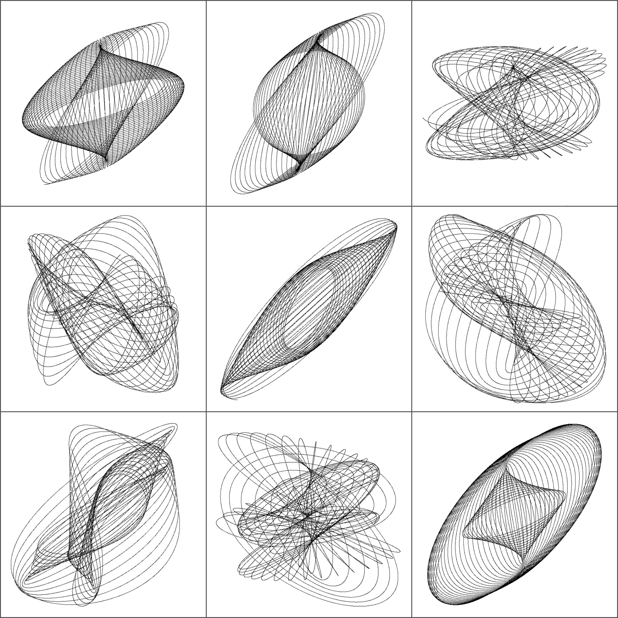
Hi, I was fascinated by the harmonographs – I remember seeing similar things done on paper on kids tv in the seventies. I took your code and extended it into 3d so I could experiment with the rgl package. I created some beautiful figures (which I would attach if this would let me). In lieu of that here is the code:

I ran his code and I was instantly fascinated: resulting curves were really beautiful. I suggested that we co-write a post and he was delighted with the idea. He proposed to me the following improvement of his own code:

I will try to create an animated gif of one figure

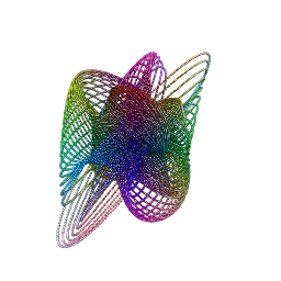
Such a good idea! And no sooner said than done: Andrew rewrote his own code to create stunning animated images of 3D-Harmonograph curves like these:

Some keys about the code:

Andrew creates 3D curves by adding a third oscillation z generated in the same way as x and y and adds a little colour by setting the colour of each point to a colour in the RGB scale related to its point in 3d space
Function spheres3d to produce an interactive plot that you can drag around to view from different angles; function spin3d will rotate the figure around the z axis and at 5 rpm in this case and function movie3d renders each frame in a temporary png file and then calls ImageMagick to stitch them into an animated gif file. It is necessary to install ImageMagick separately to create the movie.
Giving it a duration of 12 seconds at 5 rpm is one rotation which at 12 frames per second results in 144 individual png files but these (by default) are temporary and deleted when the gif is produced.

Although I don’t know Andrew personally, I know he is a good partner to work with. Thanks a lot for sharing this work of art with me and allowing me to share it in Ripples as well.

Here you have the code. I like to imagine these curves as orbits of unexplored planets in a galaxy far, far away …

library(rgl)
library(scatterplot3d)
#Extending the harmonograph into 3d
#Antonio's functions creating the oscillations
xt = function(t) exp(-d1*t)*sin(t*f1+p1)+exp(-d2*t)*sin(t*f2+p2)
yt = function(t) exp(-d3*t)*sin(t*f3+p3)+exp(-d4*t)*sin(t*f4+p4)
#Plus one more
zt = function(t) exp(-d5*t)*sin(t*f5+p5)+exp(-d6*t)*sin(t*f6+p6)
#Sequence to plot over
t=seq(1, 100, by=.001)
#generate some random inputs
f1=jitter(sample(c(2,3),1))
f2=jitter(sample(c(2,3),1))
f3=jitter(sample(c(2,3),1))
f4=jitter(sample(c(2,3),1))
f5=jitter(sample(c(2,3),1))
f6=jitter(sample(c(2,3),1))
d1=runif(1,0,1e-02)
d2=runif(1,0,1e-02)
d3=runif(1,0,1e-02)
d4=runif(1,0,1e-02)
d5=runif(1,0,1e-02)
d6=runif(1,0,1e-02)
p1=runif(1,0,pi)
p2=runif(1,0,pi)
p3=runif(1,0,pi)
p4=runif(1,0,pi)
p5=runif(1,0,pi)
p6=runif(1,0,pi)
#and turn them into oscillations
x = xt(t)
y = yt(t)
z = zt(t)
#create values for colours normalised and related to x,y,z coordinates
cr = abs(z)/max(abs(z))
cg = abs(x)/max(abs(x))
cb = abs(y)/max(abs(y))
dat=data.frame(t, x, y, z, cr, cg ,cb)
#plot the black and white version
with(dat, scatterplot3d(x,y,z, pch=16,cex.symbols=0.25, axis=FALSE ))
with(dat, scatterplot3d(x,y,z, pch=16, color=rgb(cr,cg,cb),cex.symbols=0.25, axis=FALSE ))
#Set the stage for 3d plots
# clear scene:
clear3d("all")
# white background
bg3d(color="white")
#lights...camera...
light3d()
#action
# draw shperes in an rgl window
spheres3d(x, y, z, radius=0.025, color=rgb(cr,cg,cb))
#create animated gif (call to ImageMagic is automatic)
movie3d( spin3d(axis=c(0,0,1),rpm=5),fps=12, duration=12 )
#2d plots to give plan and elevation shots
plot(x,y,col=rgb(cr,cg,cb),cex=.05)
plot(y,z,col=rgb(cr,cg,cb),cex=.05)
plot(x,z,col=rgb(cr,cg,cb),cex=.05)

Each of us has their own mappa mundi (Gala, my indispensable friend)

The harmonograph is a mechanism which, by means of several pendulums, draws trajectories that can be analyzed not only from a mathematical point of view but also from an artistic one. In its double pendulum version, one pendulum moves a pencil and the other one moves a platform with a piece of paper on it. You can see an example here. The harmonograph is easy to use: you only have to put pendulums into motion and wait for them to stop. The result are amazing undulating drawings like this one:

First harmonographs were built in 1857 by Scottish mathematician Hugh Blackburn, based on the previous work of French mathematician Jean Antoine Lissajous. There is not an unique way to describe mathematically the motion of the pencil. I have implemented the one I found in this sensational blog, where motion in both x and y axis depending on time is defined by:

$<br /> x(t)=e^{-d_{1}t}sin(f_{1}t+p_{1})+e^{-d_{2}t}sin(f_{2}t+p_{2})\\<br /> y(t)=e^{-d_{3}t}sin(f_{3}t+p_{3})+e^{-d_{4}t}sin(f_{4}t+p_{4})<br />$

I initialize parameters randomly so every time you run the script, you obtain a different output. Here is a mosaic with some of mine:

This is the code to simulate the harmonograph (no extra package is required). If you create some nice work of art, I will be very happy to admire it (you can find my email here):

f1=jitter(sample(c(2,3),1));f2=jitter(sample(c(2,3),1));f3=jitter(sample(c(2,3),1));f4=jitter(sample(c(2,3),1))
d1=runif(1,0,1e-02);d2=runif(1,0,1e-02);d3=runif(1,0,1e-02);d4=runif(1,0,1e-02)
p1=runif(1,0,pi);p2=runif(1,0,pi);p3=runif(1,0,pi);p4=runif(1,0,pi)
xt = function(t) exp(-d1*t)*sin(t*f1+p1)+exp(-d2*t)*sin(t*f2+p2)
yt = function(t) exp(-d3*t)*sin(t*f3+p3)+exp(-d4*t)*sin(t*f4+p4)
t=seq(1, 100, by=.001)
dat=data.frame(t=t, x=xt(t), y=yt(t))
with(dat, plot(x,y, type="l", xlim =c(-2,2), ylim =c(-2,2), xlab = "", ylab = "", xaxt='n', yaxt='n'))

Fronkonstin

Experiments in R

Tag Archives: beautiful

3D-Harmonographs In Motion

Beautiful Curves: The Harmonograph