Distinguishing the signal from the noise requires both scientific knowledge and self-knowledge (Nate Silver, author of The Signal and the Noise)
Analyzing the evolution of NASDAQ-100 stock prices can discover some interesting couples of companies which share a strong common trend despite of belonging to very different sectors. The NASDAQ-100 is made up of 107 equity securities issued by 100 of the largest non-financial companies listed on the NASDAQ. On the other side, Yahoo! Finance is one of the most popular services to consult financial news, data and commentary including stock quotes, press releases, financial reports, and original programming. Using R is possible to download the evolution of NASDAQ-100 symbols from Yahoo! Finance. There is a R package called quantmod which makes this issue quite simple with the function getSymbols. Daily series are long enough to do a wide range of analysis, since most of them start in 2007.
One robust way to determine if two times series, xt and yt, are related is to analyze if there exists an equation like yt=βxt+ut such us residuals (ut) are stationary (its mean and variance does not change when shifted in time). If this happens, it is said that both series are cointegrated. The way to measure it in R is running the Augmented Dickey-Fuller test, available in tseries package. Cointegration analysis help traders to design products such spreads and hedges.
There are 5.671 different couples between the 107 stocks of NASDAQ-100. After computing the Augmented Dickey-Fuller test to each of them, the resulting data frame can be converted into a distance matrix. A nice way to visualize distances between stocks is to do a hierarchical clustering. This is the resulting dendogram of the clustering:
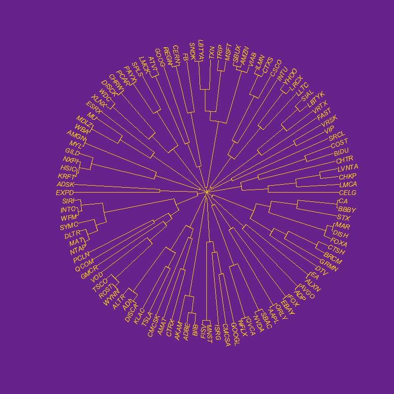
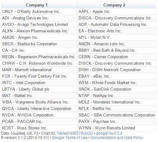
Close stocks such as Ca Inc. (CA) and Bed Bath & Beyond Inc. (BBBY) are joined with short links. A quick way to extract close couples is to cut this dendogram in a big number of clusters and keep those with two elements. Following is the list of the most related stock couples cutting dendogram in 85 clusters:
Most of them are strange neighbors. Next plot shows the evolution closing price evolution of four of these couples:

Analog Devices Inc. (ADI) makes semiconductors and Discovery Communications Inc. (DISCA) is a mass media company. PACCAR Inc. (PCAR) manufactures trucks and Paychex Inc. (PAYX) provides HR outsourcing. CA Inc. (CA) creates software and Bed Bath & Beyond Inc. (BBBY) sells goods for home. Twenty-First Century Fox Inc. (FOX) is a mass media company as well and EBAY Inc. (EBAY) does online auctions. All of them are odd connections.
This is the code of the experiment:
library("quantmod")
library("TSdist")
library("ade4")
library("ggplot2")
library("Hmisc")
library("zoo")
library("scales")
library("reshape2")
library("tseries")
library("RColorBrewer")
library("ape")
library("sqldf")
library("googleVis")
library("gridExtra")
setwd("YOUR-WORKING-DIRECTORY-HERE")
temp=tempfile()
download.file("http://www.nasdaq.com/quotes/nasdaq-100-stocks.aspx?render=download",temp)
data=read.csv(temp, header=TRUE)
for (i in 1:nrow(data)) getSymbols(as.character(data[i,1]))
results=t(apply(combn(sort(as.character(data[,1]), decreasing = TRUE), 2), 2,
function(x) {
ts1=drop(Cl(eval(parse(text=x[1]))))
ts2=drop(Cl(eval(parse(text=x[2]))))
t.zoo=merge(ts1, ts2, all=FALSE)
t=as.data.frame(t.zoo)
m=lm(ts2 ~ ts1 + 0, data=t)
beta=coef(m)[1]
sprd=t$ts1 - beta*t$ts2
ht=adf.test(sprd, alternative="stationary", k=0)$p.value
c(symbol1=x[1], symbol2=x[2], (1-ht))}))
results=as.data.frame(results)
colnames(results)=c("Sym1", "Sym2", "TSdist")
results$TSdist=as.numeric(as.character(results$TSdist))
save(results, file="results.RData")
load("results.RData")
m=as.dist(acast(results, Sym1~Sym2, value.var="TSdist"))
hc = hclust(m)
# vector of colors
op = par(bg = "darkorchid4")
plot(as.phylo(hc), type = "fan", tip.color = "gold", edge.color ="gold", cex=.8)
# cutting dendrogram in 85 clusters
clusdf=data.frame(Symbol=names(cutree(hc, 85)), clus=cutree(hc, 85))
clusdf2=merge(clusdf, data[,c(1,2)], by="Symbol")
sizes=sqldf("SELECT * FROM (SELECT clus, count(*) as size FROM clusdf GROUP BY 1) as T00 WHERE size>=2")
sizes2=merge(subset(sizes, size==2), clusdf2, by="clus")
sizes2$id=sequence(rle(sizes2$clus)$lengths)
couples=merge(subset(sizes2, id==1)[,c(1,3,4)], subset(sizes2, id==2)[,c(1,3,4)], by="clus")
couples$"Company 1"=apply(couples[ , c(2,3) ] , 1 , paste , collapse = " -" )
couples$"Company 2"=apply(couples[ , c(4,5) ] , 1 , paste , collapse = " -" )
CouplesTable=gvisTable(couples[,c(6,7)])
plot(CouplesTable)
# Plots
opts2=theme(
panel.background = element_rect(fill="gray98"),
panel.border = element_rect(colour="black", fill=NA),
axis.line = element_line(size = 0.5, colour = "black"),
axis.ticks = element_line(colour="black"),
panel.grid.major = element_line(colour="gray75", linetype = 2),
panel.grid.minor = element_blank(),
axis.text = element_text(colour="gray25", size=12),
axis.title = element_text(size=18, colour="gray10"),
legend.key = element_rect(fill = "white"),
legend.text = element_text(size = 14),
legend.background = element_rect(),
plot.title = element_text(size = 35, colour="gray10"))
plotPair = function(Symbol1, Symbol2)
{
getSymbols(Symbol1)
getSymbols(Symbol2)
close1=Cl(eval(parse(text=Symbol1)))
close2=Cl(eval(parse(text=Symbol2)))
cls=merge(close1, close2, all = FALSE)
df=data.frame(date = time(cls), coredata(cls))
names(df)[-1]=c(Symbol1, Symbol2)
df1=melt(df, id.vars = "date", measure.vars = c(Symbol1, Symbol2))
ggplot(df1, aes(x = date, y = value, color = variable))+
geom_line(size = I(1.2))+
scale_color_discrete(name = "")+
scale_x_date(labels = date_format("%Y-%m-%d"))+
labs(x="Date", y="Closing Price")+
opts2
}
p1=plotPair("ADI", "DISCA")
p2=plotPair("PCAR", "PAYX")
p3=plotPair("CA", "BBBY")
p4=plotPair("FOX", "EBAY")
grid.arrange(p1, p2, p3, p4, ncol=2)
Nice post.
Your regression seems to be on closing prices
ts1=drop(Cl(eval(parse(text=x[1]))))
ts2=drop(Cl(eval(parse(text=x[2]))))
t.zoo=merge(ts1, ts2, all=FALSE)
t=as.data.frame(t.zoo)
m=lm(ts2 ~ ts1 + 0, data=t)
Perhaps repeat on the return on closing prices instead.
e.g. drop(ROC(Cl( …. or something similar
Aside: difficult to read the code as there is no formatting e.g. indentation. Would be easier to read if wordpress would allow this to be preserved.
Great post.
… but the code is extremely difficult to read. Using
– piping (http://cran.r-project.org/web/packages/magrittr/vignettes/magrittr.html)
– dplyr (http://cran.rstudio.com/web/packages/dplyr/vignettes/introduction.html) instead of subset(sizes2, id==1)[,c(1,3,4)] etc..
– some comments
– spacing/formatting within functions and for() cycles
could turn into readable and easy to follow fantastic post!
Thanks, you a re right. I need to improve the code to make it more readable. I promise doing my best!
While trying to follow your code line by line, I have one more comment, besides using a regression on price returns instead of price time series itself, you were building a wrong spread:
m=lm(ts2 ~ ts1 + 0, data=t)
beta=coef(m)[1]
sprd=t$ts1 – beta*t$ts2 #mistake here
The spread should be sprd=t$ts2 – beta*t$ts1, since you ts2 is the response and ts1 is the predictor.
You can actually get the spread from the model by using the function residuals(). residuals(m) == t$ts2 – beta*t$ts1 in your case.
Thanks, I will check it out
I might suggest that the results variable should look something like that:
require(magrittr)
require(dplyr)
dataPairs %
arrange(., desc(Symbol)) %>% #sort in descending order
select(.,Symbol) %>% # take only the Symbols column
t() %>% # transpose
combn(.,2) # build combinations of pairs
results=t(apply(dataPairs, 2,
function(x) {
ts1 %
parse(text = .) %>%
eval() %>% #fetching price martix
Cl() %>% #selecting “Close” prices only
drop() %>%
log() %>% # diff(log()) would give us log returns
diff()
ts2 %
parse(text = .) %>%
eval() %>%
Cl() %>%
drop() %>%
log() %>%
diff()
t %
na.omit() %>% #removing first row of NAs
as.data.frame()
m=lm(ts2 ~ ts1, data=t)
ht=adf.test(residuals(m), alternative=”stationary”, k=0)$p.value
c(symbol1=x[1], symbol2=x[2], (1-ht))
}
)
)
But if I run the code above, I get results$TSdist all equal to 0.99
It is appropriate that you have quoted Nate Silver at the beginning.
It appears that you have painstakingly searched and found noise in the data. When you have 100+ different stocks, by chance alone you will find high correlation between a few stocks, even though the stocks have no relation.
I have disected one of your posts codings to see how you do your workflow. But I wonder how you chose your combination of packages? Do you know a lot of them or do you search each time you have a certain need?
The one you have disected is a bit messy. At the beginning I used to search intensely each time but know I don’t sopend so many doing that. The more you use R the more you know.