The chess-board is the world; the pieces are the phenomena of the universe; the rules of the game are what we call the laws of Nature (T. H. Huxley)
One of the greatest packages I discovered recently is googleVis. While plotting with ggplot can be sometimes very arduous, doing plots with googleVis is extremely easy. Here you can find many examples of what you can do with this great package.
Not long ago, I also discovered The On-Line Encyclopedia of Integer Sequences (OEIS), a huge database of about 250.000 integer sequences where, for example, you can find the number of ways to lace a shoe that has n pairs of eyelets or the smallest number of stones in Tchoukaillon (or Mancala, or Kalahari) solitaire which make use of n-th hole. Many mathematicians, as Ralph Stephan, use this useful resource to develop their theories.
The third protagonist of this story is Frank Benford, who formulated in 1938 his famous law which states that considering different lists of numbers, 1 occurs as the leading digit about the 30% of time, while larger digits occur in that position less frequently.
In this experiment I read 20 random sequences from the OEIS. For each sequence, I obtain the distribution of first digit of the numbers and calculate the similarity with the theoretical distribution given by Benford’s Law so the more similar is the distribution, the closer is this number to 1. Sequences of OEIS are labeled with a seven characters code (an “A” followed by 6 digits). A nice way to show the output of this experiment is using the Gauge visualization of googleVis:
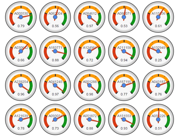
Sequence A001288 is the closest to the Benford’s Law. This sequence is the number of distinct 11-element subsets that can be formed from a n element set. Why is so close to the Benford’s Law? No idea further than binomial coefficients are related to some biological laws as number of descendants of a couple of rabbits.
I would like to wish you all a Merry Christmas and a Happy New Year:
library(plyr)
bendford=data.frame(first=0:9, freq=c(0,log10(1+1/(1:9))))
SequencesIds=formatC(sample(1:250000, 20, replace=FALSE), width = 6, format = "d", flag = "0")
results=data.frame(SEQID=character(0), BENDFORNESS=numeric(0))
for(i in 1:length(SequencesIds))
{
  SEQID = SequencesIds[i]
  TEXTFILE=paste("b", SEQID, ".txt", sep="")
  if (!file.exists(TEXTFILE)) download.file(paste("http://oeis.org/A",SEQID, "/b", SEQID, ".txt",sep=""), destfile = TEXTFILE)
  SEQ=readLines(paste("b", SEQID, ".txt", sep=""))
  SEQ=SEQ[SEQ != ""]
  SEQ=SEQ[unlist(gregexpr(pattern ='synthesized',SEQ))<0]
  m=t(sapply(SEQ, function(x) unlist(strsplit(x, " "))))
  df=data.frame(first=substr(gsub("[^0-9]","",m[,2]), 1, 1), row.names = NULL)
  df=count(df, vars = "first")
  df$freq=df$freq/sum(df$freq)
  df2=merge(x = bendford, y = df, by = "first", all.x=TRUE)
  df2[is.na(df2)]=0
  results=rbind(results, data.frame(SEQID=paste("A", SEQID, sep=""), BENDFORNESS=1-sqrt(sum((df2$freq.x - df2$freq.y) ^ 2))))
}
results$BENDFORNESS=as.numeric(format(round(results$BENDFORNESS, 2), nsmall = 2))
Gauge=gvisGauge(results, options=list(min=0, max=1, greenFrom=.75, greenTo=1, yellowFrom=.25, yellowTo=.75, redFrom=0, redTo=.25, width=400, height=300))
plot(Gauge)
Hi, thank you for doing this.
Maybe it would be useful set.seed for reproducibility
I got 0.99 on my first try with A206171
Merry Christmas!
Rafa
You are welcome. Without set.seeding maybe someone will find interesting results …
Ok, respectufully the gauges are horrible: they impair comparison and prevent rapid perception of the information displayed. Please consider using a horizontal (sorted) bar graph or better a dot plot http://www.statmethods.net/graphs/dot.html
Thanks for your comment. I think gauges are useful in some contexts as dashboarding or qualitative comparisons. This is a post about how to use googleVis and I chose this visualization because I like the effect of “a grid of gauges” and because this kind of charts are underused from my point of view. I like them. Regards.
Have you tried playing with bullet graphs? I believe there is an R package for it: http://statistik-stuttgart.de/bullet-graph-in-r/
Also suggests reading this:
http://www.amazon.com/Information-Dashboard-Design-At—Glance/dp/1938377001/ref=asap_bc?ie=UTF8
and this:
https://www.google.ca/url?sa=t&rct=j&q=&esrc=s&source=web&cd=2&ved=0CC4QFjAB&url=https%3A%2F%2Fweb.cs.dal.ca%2F~sbrooks%2Fcsci4166-6406%2Fseminars%2Freadings%2FCleveland_GraphicalPerception_Science85.pdf&ei=LCW3VOmuEMy8yQTerYDoDA&usg=AFQjCNEtm8_6q3-uHUGRVTYEG0TT17JA-w&sig2=mfdPHl_RUlytj-Nf8ovu9A&bvm=bv.83640239,d.aWw&cad=rja