Category Archives: Sports Analytics

A Checkpoint Of Spanish Football League

I am an absolute beginner, but I am absolutely sane (Absolute Beginners, David Bowie)

Some time ago I wrote this post, where I predicted correctly the winner of the Spanish Football League several months before its ending. After thinking intensely about taking the risk of ruining my reputation repeating the analysis, I said “no problem, Antonio, do it again: in the end you don’t have any reputation to keep”. So here we are.

From a technical point of view there are many differences between both analysis. Now I use webscraping to download data, dplyr and pipes to do transformations and interactive D3.js graphs to show results. I think my code is better now and it makes me happy.

As I did the other time, Bradley-Terry Model gives an indicator of  the power of each team, called ability, which provides a natural mechanism for ranking teams. This is the evolution of abilities of each team during the championship (last season was played during the past weekend):

liga1_ability2

Although it is a bit messy, the graph shows two main groups of teams: on the one hand, Barcelona, Atletico de Madrid, Real Madrid and Villareal; on the other hand, the rest. Let’s have a closer look to evolution of the abilities of the top 4 teams:

liga2_ability2

While Barcelona, Atletico de Madrid and Real Madrid walk in parallel,  Villareal seems to be a bit stacked in the last seasons; the gap between them and Real Madrid is increasing little by little. Maybe is the Zidane’s effect. It is quite interesting discovering what teams are increasing their abilities: they are Malaga, Eibar and Getafe. They will probably finish the championship in a better position than they have nowadays (Eibar could reach fifth position):

liga3_ability2

What about Villareal? Will they go up some position? I don’t think so. This plot shows the probability of winning any of the top 3:

liga4_villareal2

As you can see, probability is decreasing significantly. And what about Barcelona? Will win? It is a very difficult question. They are almost tied with Atletico de Madrid, and only 5 and 8 points above Real Madrid and Villareal. But it seems Barcelona keep them at bay. This plot shows the evolution of the probability of be beaten by Atletico, Real Madrid and Villareal:

liga5_Barcelona2

All probabilities are under 50% and decreasing (I supposed a scoring of 2-0 for Barcelona in the match against Sporting of season 16 that was postponed to next February 17th).

Data science is a profession for brave people so it is time to do some predictions. These are mine, ordered by likelihood:

  • Barcelona will win, followed by Atletico (2), Real Madrid (3), Villareal (4) and Eibar (5)
  • Malaga and Getafe will go up some positions
  • Next year I will do the analysis again

Here you have the code:

library(rvest)
library(stringr)
library(BradleyTerry2)
library(dplyr)
library(reshape)
library(rCharts)
nseasons=20
results=data.frame()
for (i in 1:nseasons)
{
  webpage=paste0("http://www.marca.com/estadisticas/futbol/primera/2015_16/jornada_",i,"/")
  html(webpage) %>%
    html_nodes("table") %>%
    .[[1]] %>%
    html_table(header=FALSE, fill=TRUE) %>%
    mutate(X4=i) %>%
    rbind(results)->results
}
colnames(results)=c("home", "score", "visiting", "season")
results %>% 
  mutate(home     = iconv(home,     from="UTF8",to="ASCII//TRANSLIT"),
         visiting = iconv(visiting, from="UTF8",to="ASCII//TRANSLIT")) %>%
  #filter(grepl("-", score)) %>%
  mutate(score=replace(score, score=="18:30 - 17/02/2016", "0-2")) %>% # resultado fake para el Barcelona
  mutate(score_home     = as.numeric(str_split_fixed(score, "-", 2)[,1])) %>%
  mutate(score_visiting = as.numeric(str_split_fixed(score, "-", 2)[,2])) %>%
  mutate(points_home     =ifelse(score_home > score_visiting, 3, ifelse(score_home < score_visiting, 0, 1))) %>%
  mutate(points_visiting =ifelse(score_home > score_visiting, 0, ifelse(score_home < score_visiting, 3, 1))) -> data
prob_BT=function(x, y) {exp(x-y) / (1 + exp(x-y))}
BTabilities=data.frame()
for (i in 13:nseasons)
{
  data %>% filter(season<=i) %>%
    BTm(cbind(points_home, points_visiting), home, visiting, data=.) -> footballBTModel
  BTabilities(footballBTModel) %>%
  as.data.frame()  -> tmp 
  cbind(tmp, as.character(rownames(tmp)), i) %>% 
  mutate(ability=round(ability, digits = 2)) %>%
  rbind(BTabilities) -> BTabilities
}
colnames(BTabilities)=c("ability", "s.e.", "team", "season")
sort(unique(BTabilities[,"team"])) -> teams
BTprobabilities=data.frame()
for (i in 13:nseasons)
{
  BTabilities[BTabilities$season==i,1] %>% outer( ., ., prob_BT) -> tmp
  colnames(tmp)=teams
  rownames(tmp)=teams  
  cbind(melt(tmp),i) %>% rbind(BTprobabilities) -> BTprobabilities
}
colnames(BTprobabilities)=c("team1", "team2", "probability", "season")
BTprobabilities %>% 
  filter(team1=="Villarreal") %>% 
  mutate(probability=round(probability, digits = 2)) %>%
  filter(team2 %in% c("R. Madrid", "Barcelona", "Atletico")) -> BTVillareal
BTprobabilities %>% 
  filter(team2=="Barcelona") %>% 
  mutate(probability=round(probability, digits = 2)) %>%
  filter(team1 %in% c("R. Madrid", "Villarreal", "Atletico")) -> BTBarcelona
AbilityPlot <- nPlot(
  ability ~ season, 
  data = BTabilities, 
  group = "team",
  type = "lineChart")
AbilityPlot$yAxis(axisLabel = "Estimated Ability", width = 62)
AbilityPlot$xAxis(axisLabel = "Season")
VillarealPlot <- nPlot(
  probability ~ season, 
  data = BTVillareal, 
  group = "team2",
  type = "lineChart")
VillarealPlot$yAxis(axisLabel = "Probability of beating", width = 62)
VillarealPlot$xAxis(axisLabel = "Season")
BarcelonaPlot <- nPlot(
  probability ~ season, 
  data = BTBarcelona, 
  group = "team1",
  type = "lineChart")
BarcelonaPlot$yAxis(axisLabel = "Probability of being beaten", width = 62)
BarcelonaPlot$xAxis(axisLabel = "Season")
Analysing The Rock ‘n’ Roll Madrid Marathon

Nobody’s going to win all the time. On the highway of life you can’t always be in the fast lane (Haruki Murakami, What I Talk About When I Talk About Running)

I started running two years ago and one if my dreams is to run a marathon someday. One month ago I run my first half marathon so this day is become closer but I am in no hurry to do it. Meanwhile, I prefer analysing the results of the last edition of the Rock ‘n’ Roll Madrid marathon which, by the way, will be hold again next weekend. This is the first time I do webscraping to download data from a website and it has been quite easy thanks to rvest package.

Once I go over this website form, I have timings of every runner (more than 11.000) at 5, 10, 15, 20, 21.097, 25, 30, 35, 40, and 42.195 kilometers. This, togheter with the category of each runner is the base for my analysis. I remove categories with a small number of runners.

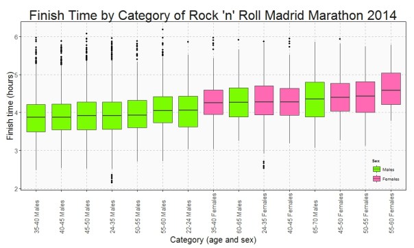
This is the Box plot of the finish time by category:

Finish Time

Who maintains the rhythm better? Since I have the time at the end and at the middle (21.097 km), I can do a Box plot with the variation time between first and second half of the Marathon:

Variation Time

Only a handful of people pull out of the Marathon before finishing but once again this rate is not the same between categories. This is the survival rate by category along the race:

Survival Rate

This plots show some interesting things:

  • Fastest category is 35-40 years old for both genders
  • Fastest individuals are inside 24-35 years old for both genders
  • Youngest ages are not the fastest
  • Between 40-45 category is the second fastest for men and the third one for women
  • Females between 40-45 keep the most constant rhythm of all categories.
  • Young men between 22-24 years old are the most unconstant: their second half rhythm is much slower than the first one.
  • All females between 55-60 years old ended the marathon
  • On the other hand, males between 60-65 are the category with most ‘deads’ during the race

Long life forties:

library(rvest)
library(lubridate)
library(ggplot2)
library(plyr)
library(sqldf)
library(scales)
library(gplots)
setwd("YOUR WORKING DIRECTORY HERE")
maraton_web="http://www.maratonmadrid.org/resultados/clasificacion.asp?carrera=13&parcial=par1&clasificacion=1&dorsal=&nombre=&apellidos=&pais=&pagina=par2"
#Grid with parameters to navigate in the web to do webscraping
searchdf=rbind(expand.grid( 1, 0:32), expand.grid( 2, 0:55), expand.grid( 3, 0:56), expand.grid( 4, 0:56),
               expand.grid( 5, 0:56), expand.grid( 6, 0:55), expand.grid( 7, 0:55), expand.grid( 8, 0:55),
               expand.grid( 9, 0:53), expand.grid(10, 0:55))
colnames(searchdf)=c("parcial", "pagina")
#Webscraping. I open the webpage and download the related table with partial results
results=data.frame()
for (i in 1:nrow(searchdf))
{
  maraton_tmp=gsub("par2", searchdf[i,2], gsub("par1", searchdf[i,1], maraton_web))
  df_tmp=html(maraton_tmp) %>% html_nodes("table") %>% .[[3]] %>% html_table()
  results=rbind(results, data.frame(searchdf[i,1], df_tmp[,1:7]))
}
#Name the columns
colnames(results)=c("Partial", "Place", "Bib", "Name", "Surname", "Cat", "Gross", "Net")
#Since downloadind data takes time, I save results in RData format
save(results, file="results.RData")
load("results.RData")
#Translate Net timestamp variable into hours
results$NetH=as.numeric(dhours(hour(hms(results$Net)))+dminutes(minute(hms(results$Net)))+dseconds(second(hms(results$Net))))/3600
results$Sex=substr(results$Cat, 3, 4)
#Translate Cat into years and gender
results$Cat2=revalue(results$Cat, 
                     c("A-F"="18-22 Females", "A-M"="18-22 Males", "B-F"="22-24 Females", "B-M"="22-24 Males", "C-F"="24-35 Females", "C-M"="24-35 Males", 
                       "D-F"="35-40 Females", "D-M"="35-40 Males", "E-F"="40-45 Females", "E-M"="40-45 Males", "F-F"="45-50 Females", "F-M"="45-50 Males", 
                       "G-F"="50-55 Females", "G-M"="50-55 Males", "H-F"="55-60 Females", "H-M"="55-60 Males", "I-F"="60-65 Females", "I-M"="60-65 Males", 
                       "J-F"="65-70 Females", "J-M"="65-70 Males", "K-F"="+70 Females", "K-M"="+70 Males"))
#Translate partial code into kilometers
results$PartialKm=mapvalues(results$Partial, from = c(1, 2, 3, 4, 5, 6, 7, 8, 9, 10), to = c(5, 10, 15, 20, 21.097, 25, 30, 35, 40, 42.195))
#There are some categories with very few participants. I will remove from the analysis
count(subset(results, Partial==10), "Cat")
#General options for ggplot
opts=theme(
  panel.background = element_rect(fill="gray98"),
  panel.border = element_rect(colour="black", fill=NA),
  axis.line = element_line(size = 0.5, colour = "black"),
  axis.ticks = element_line(colour="black"),
  panel.grid.major = element_line(colour="gray75", linetype = 2),
  panel.grid.minor = element_blank(),
  axis.text = element_text(colour="gray25", size=15),
  axis.title = element_text(size=20, colour="gray10"),
  legend.key = element_blank(),
  legend.background = element_blank(),
  plot.title = element_text(size = 32, colour="gray10"))
#Data set with finish times
results1=subset(results, Partial==10 & !(Cat %in% c("A-F", "A-M", "B-F", "I-F", "J-F", "K-F", "K-M")))
ggplot(results1, aes(x=reorder(Cat2, NetH, FUN=median), y=NetH)) + geom_boxplot(aes(fill=Sex), colour = "gray25")+
  scale_fill_manual(values=c("hotpink", "lawngreen"), name="Sex", breaks=c("M", "F"), labels=c("Males", "Females"))+
  labs(title="Finish Time by Category of Rock 'n' Roll Madrid Marathon 2014", x="Category (age and sex)", y="Finish time (hours)")+
  theme(axis.text.x = element_text(angle = 90, vjust=.5, hjust = 0), legend.justification=c(1,0), legend.position=c(1,0))+opts
#Data set with variation times
results2=sqldf("SELECT 
               a.Bib, a.Sex, b.Cat2, (a.NetH-2*b.NetH)*60 as VarMin
               FROM results1 a INNER JOIN results b ON (a.Bib = b.Bib AND b.Partial=5) order by VarMin asc")
ggplot(results2, aes(x=reorder(Cat2, VarMin, FUN=median), y=VarMin)) + geom_boxplot(aes(fill=Sex))+
  scale_fill_manual(values=c("hotpink", "lawngreen"), name="Sex", breaks=c("M", "F"), labels=c("Males", "Females"))+
  labs(title="Time Variation by Category Between First and Last Half\nof Rock 'n' Roll Madrid Marathon 2014", x="Category (age and sex)", y="Variation (minutes)")+
  theme(axis.text.x = element_text(angle = 90, vjust=.5, hjust = 0), legend.justification=c(1,0), legend.position=c(1,0))+opts
 
results3_tmp1=expand.grid(Cat2=unique(results$Cat2), PartialKm=unique(results$PartialKm))
results3_tmp2=sqldf("SELECT Bib, Sex, Cat2, Max(PartialKm) as PartialKmMax FROM results 
                   WHERE Cat NOT IN ('A-F', 'A-M', 'B-F', 'I-F', 'J-F', 'K-F', 'K-M') GROUP BY 1,2,3")
results3_tmp3=sqldf("SELECT PartialKmMax, Sex, Cat2, COUNT(*) AS Runners FROM results3_tmp2 GROUP BY 1,2,3")
results3_tmp4=sqldf("SELECT a.Cat2, a.PartialKm, SUM(Runners) as Runners FROM results3_tmp1 a INNER JOIN results3_tmp3 b
                    on (a.Cat2 = b.Cat2 AND b.PartialKmMax>=a.PartialKm) 
                    GROUP BY 1,2")
#Data set with survival rates
results3=sqldf("SELECT a.Cat2, a.PartialKm, a.Runners*1.00/b.Runners*1.00 as Po_Survivors
               FROM results3_tmp4 a INNER JOIN (SELECT Cat2, COUNT(*) as Runners FROM results3_tmp2 GROUP BY 1) b
               ON (a.Cat2 = b.Cat2)")
ggplot(results3, aes(x=PartialKm, y=Po_Survivors, group=Cat2, colour=Cat2)) + geom_line(lwd=3)+
  scale_color_manual(values=alpha(rich.colors(15, palette="temperature"), 0.3), name="Category")+
  scale_x_continuous(breaks = unique(results3$PartialKm), labels=c("5", "10", "15", "20", "21.097", "25", "30", "35", "40", "42.195"))+
  scale_y_continuous(labels = percent)+
  labs(title="Survival Rate by Category of Rock 'n' Roll Madrid Marathon 2014", x="Kilometer", y="% of survivors")+
  theme(axis.text.x = element_text(angle = 90, vjust=.5, hjust = 0), legend.justification=c(1,0), legend.position=c(.15,0))+opts

Why I Think Atletico De Madrid Will Win 2013/14 Spanish Liga Of Football

Prediction is difficult, especially of the future (Mark Twain)

Let me start with two important premises. First of all, I am not into football so I do not support any team. Second, this post is just an opinion based on mathematics but football, as all of you know, is not an exact science. Football is football.

This is a good moment to analyse Spanish Liga of football. F. C. Barcelona and Atletico de Madrid share first place of the championship followed closely by Real Madrid. But analysing results over the time can give us an interesting insight about capabilities of top three teams.

I have run a Bradley-Terry model for pairwise comparisons. The Bradley-Terry model deals with a situation in which n individuals or items are compared to one another in paired contests. In my case the model uses confrontations and its results as input. The Bradley-Terry model (Bradley and Terry 1952) assumes that in a contest between any two players, say player i and player j, the odds that i beats j are xi/xj, where xi and xj are positive-valued parameters which might be thought of as representing ability.

Time plays a key role in my analysis. This is what happens when you estimate abilities of top three teams over the time:

abilities

After 20 rounds, Atletico de Madrid and Barcelona have the same estimated ability but while Barcelona is continuosly losing ability since the beginning, Atletico de Madrid presents a robust or even growing evolution. Of course, it depends on how both teams begun the championship. The higher you start, the more you can lose; but watching this graph I can not help feeling that Atletico de Madrid keep their morale higher than Barcelona.

Another interesting output of  the Bradley-Terry model are estimated probabilites of beating teams each others. Since these probabilities depends on previous abilities, Barcelona and Atletico de Madrid have same chances of winning a hypothetical match. But once again, evolution of these probabilities can change our perception:

probabilities

As you can see, Atletico de Madrid has increased the probability of beating Barcelona from 0.25 to 0.50 in just one round and Barcelona has lost more than this probability in the same time. Once again, it seems that Atletico de Madrid is increasingly confidence time by time. And confidence is important in this game. Luckily, football is unpredictable but after taking time into account I dare to say that Atletico de Madrid will win the championship. I am pretty sure.

Here you have the code I wrote for the analysis. Maybe you would like to make your own predictions:

library("BradleyTerry2")
library("xlsx")
library("ggplot2")
library("reshape")
football <-read.xlsx("CalendarioLiga2013-14 2.xls", sheetName= "results", header=TRUE)
inv_logit <- function(p) {exp(p) / (1 + exp(p))}
prob_BT   <- function(ability_1, ability_2) {inv_logit(ability_1 - ability_2)}
rounds <- sort(unique(football$round))
# Initialization
football.pts.ev <- as.data.frame(c())
football.abl.ev <- as.data.frame(c())
football.prb.ev <- as.data.frame(c())
# Points evolution: football.pts.ev
for (i in 1:length(rounds))
{
  football.home <-aggregate( home.wins ~ home.team, data=football[football$round<=rounds[i],], FUN=sum)
  colnames(football.home) <- c('Team', 'Points')
  football.away <-aggregate( away.wins ~ away.team, data=football[football$round<=rounds[i],], FUN=sum)
  colnames(football.away) <- c('Team', 'Points')
  football.all <-rbind(football.home,football.away)
  football.points <-aggregate( Points ~ Team, data=football.all, FUN=sum)
  football.points$round<-rounds[i]
  football.pts.ev <- rbind(football.points, football.pts.ev)
}
# BT Models 
# Abilities and probabilities evolution: football.abl.ev and football.prb.ev
# We start from 6th. round to have good information
for (i in 6:length(rounds))
{
  footballBTModel      <- BTm(cbind(home.wins, away.wins), home.team, away.team, data = football[football$round<=rounds[i],], id = "team")
  team_abilities       <- data.frame(BTabilities(footballBTModel))$ability 
  names(team_abilities) <-unlist(attr(BTabilities(footballBTModel), "dimnames")[1][1])
  team_probs           <- outer(team_abilities, team_abilities, prob_BT) 
  diag(team_probs)     <- 0 
  team_probs           <- melt(team_probs)
  colnames(team_probs) <- c('team', 'adversary', 'probability')
  team_probs$round<-rounds[i]
  football.prb.ev <- rbind(team_probs, football.prb.ev)
  football.abl.ev.df <- data.frame(rownames(data.frame(BTabilities(footballBTModel))),BTabilities(footballBTModel))
  football.abl.ev.df$round<-rounds[i]
  colnames(football.abl.ev.df) <- c('team', 'ability', 's.e.', 'round')
  football.abl.ev <- rbind(football.abl.ev.df, football.abl.ev)
}
# Probabilities of top 3 teams
football.prb.ev.3 <- football.prb.ev[
    ((football.prb.ev$team == "At. Madrid" & football.prb.ev$adversary == "R. Madrid")|
     (football.prb.ev$team == "At. Madrid" & football.prb.ev$adversary == "Barcelona")|
     (football.prb.ev$team == "Barcelona"  & football.prb.ev$adversary == "R. Madrid"))&
      football.prb.ev$round>=10, ]
football.prb.ev.3$teambyadver <- interaction(football.prb.ev.3$team, football.prb.ev.3$adversary, sep = " Beating ")
# Abilities of top 3 teams
football.abl.ev.3 <- football.abl.ev[(football.abl.ev$team == "At. Madrid" | 
                                     football.abl.ev$team == "R. Madrid"  | 
                                     football.abl.ev$team == "Barcelona")&
                                     football.abl.ev$round>=10, ]
ggplot(data = football.prb.ev.3, aes(x = round, y = probability, colour = teambyadver)) +  
  stat_smooth(method = "loess", formula = y ~ x, size = 1, alpha = 0.25)+
  geom_point(size = 4) +
  theme(legend.position = c(.75, .15))+
  labs(list(x = "Round", y = "Probability"))+
  labs(colour = "Probability of ...")+
  ggtitle("Evolution Of Beating Probabilities \nAmong Top 3 First-Team") + 
  theme(plot.title = element_text(size=25, face="bold"))+
  scale_x_continuous(breaks = c(10,11,12,13,14,15,16,17,18,19,20))
ggplot(data = football.abl.ev.3, aes(x = round, y = ability, colour = team)) +  
  stat_smooth(method = "loess", formula = y ~ x, size = 1, alpha = 0.25)+
  geom_point(size = 4) +
  theme(legend.position = c(.75, .75))+
  labs(list(x = "Round", y = "Ability"))+
  labs(colour = "Ability of ...")+
  ggtitle("Evolution Of Abilities \nOf Top 3 First-Team") + 
  theme(plot.title = element_text(size=25, face="bold"))+
  scale_x_continuous(breaks = c(10,11,12,13,14,15,16,17,18,19,20))